I was standing in a German automotive supplier's conference room when their quality director explained why their latest sensor batch was failing. The units had operated flawlessly for eighteen months, then began failing in the field. The root cause was electrolyte evaporation in a capacitor operating at full temperature. This was not a manufacturing defect but an underestimated degradation mechanism.
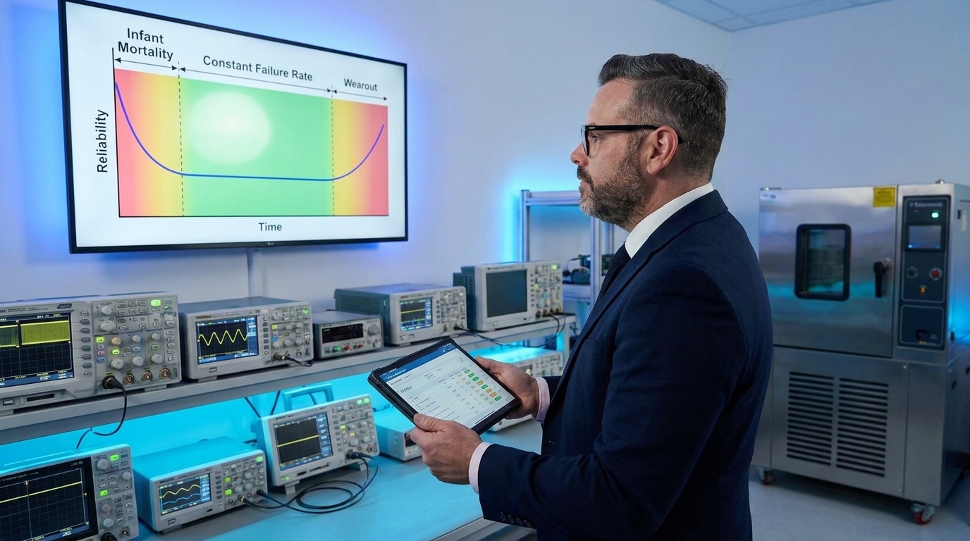
That investigation reinforced a fundamental principle of reliability engineering: if you do not understand the bathtub curve, you cannot manage product reliability. The model maps failure rates across three distinct lifecycle phases, each demanding a radically different quality response.
Mixing up these phases leads to costly mistakes. You end up applying statistical process control to a wear-out problem, or scheduling preventive maintenance for components suffering from infant mortality. Matching the engineering tool to the correct lifecycle phase is what separates reactive firefighting from systematic quality management.
Infant Mortality: Exposing Systematic Process Weaknesses
The first phase of the bathtub curve shows a high initial failure rate that drops sharply over time. These failures stem from manufacturing defects, weak components, improper assembly, or inadequate quality control. They are not random. They are systematic symptoms of an imperfect production process.
Consider an automotive lighting module line where 150 parts per 10,000 fail within the first three weeks. Root causes typically include insufficient solder reflow profiles, improperly bonded optical elements, or micro-cracks in housings that only appear during the first thermal stress cycle. Each failure represents a process escape that final inspection missed.
Because these early failures usually fall under warranty coverage, they directly erode profit margins. The countermeasures are well-established in IATF 16949 environments. Environmental Stress Screening (ESS), targeted burn-in testing, and rigorous statistical process control at critical operations force weak units to fail inside your factory rather than at the customer's plant.
Implementing 100 percent end-of-line testing for safety-critical parts catches assembly defects before shipment. However, screening alone is insufficient. The ultimate goal is traceability: using the failure data from burn-in tests to drive PFMEA updates and tighten process tolerances upstream, eliminating the defect at its source.
Useful Life and the Mathematics of Constant Failure
In the second phase, the failure rate flattens and stabilises. Failures occur randomly, caused by unpredictable environmental events, extreme operating conditions, or inherent statistical variability. This flat baseline represents the product performing exactly as designed under normal operating parameters.
During this useful life period, reliability calculations assume an exponential distribution governed by the failure rate parameter, lambda. The Mean Time Between Failures (MTBF) is simply the inverse of this rate. This mathematical relationship is the foundation of warranty cost forecasting and maintenance scheduling.
This is where field performance meets contractual obligations. If your failure rate here is too high, warranty claims escalate and brand reputation degrades. If the failure rate is remarkably low, you may be over-engineering the product, spending excessive capital on redundant component ratings that offer no marketable value.
MTBF is a population average, not a guaranteed lifespan for every individual unit on the line.
A persistent misunderstanding in engineering teams treats MTBF as a minimum product lifespan. A 50,000-hour MTBF does not mean a specific unit will survive 50,000 hours of continuous operation. It means that across a large population of identical units, failures will average out to one event per 50,000 hours of aggregate operation time.
| Metric | Description | Engineering Significance |
|---|---|---|
| MTBF | Mean Time Between Failures | Baseline metric for repairable system reliability and maintenance scheduling. |
| MTTF | Mean Time To Failure | Standard metric for non-repairable system components and materials. |
| Failure Rate (λ) | Failures per unit of time | The core parameter driving the exponential distribution model. |
| Reliability R(t) | Probability of survival over time | Calculated as R(t) = e^(-λt), defining warranty exposure. |
Wear-out: Inevitable Physical Degradation
The third phase sees the failure rate climb steeply. Mechanical components wear down, elastomers harden, and electrical contacts degrade. This is not a defect or a quality escape. It is the physical reality of a product reaching the end of its engineered lifespan.
Returning to the German sensor supplier: the capacitors performed as specified for eighteen months before the electrolyte evaporation accelerated. The root cause was not a manufacturing flaw but an underestimation of operating temperatures during the design phase. The component was dimensioned perfectly for lab conditions but failed under actual engine bay thermal loads.
You cannot inspect your way out of the wear-out phase. The engineering responses are strictly proactive. Predictive maintenance, vibration analysis, thermal monitoring, and accelerated life testing help anticipate component end-of-life. The objective is to replace critical parts during planned downtime before they fail catastrophically in the field.
Weibull analysis is the definitive statistical tool for characterising this phase. By modelling time-to-failure data, engineers can pinpoint exactly when wear-out begins to accelerate. This allows organisations to schedule component replacement intervals with absolute confidence, maximising useful life without risking field failures.
Using Weibull Analysis to Diagnose Failure Phases
Weibull distribution translates raw failure data into actionable lifecycle diagnostics. The shape parameter, beta, immediately tells you which section of the bathtub curve your product occupies, directing your engineering response with mathematical certainty.
When beta is less than one, failures are decreasing. You have an infant mortality problem, meaning a manufacturing process or a component supplier is out of control. When beta equals one, failures are random and constant. You are in the useful life phase. When beta exceeds one, failures are increasing, indicating that physical wear-out mechanisms have taken hold.
I analysed field returns for a brake sensor batch that yielded a beta of 0.7. This low value confirmed a manufacturing defect rather than a design flaw. The investigation revealed that a sub-supplier had changed their solder alloy composition without approval. The unauthorised substitution was generating internal stress fractures during the initial thermal cycling.
Interpreting the Weibull Shape Parameter (Beta)
What teams often assume
- All field returns indicate a design or manufacturing flaw.
- Warranty claims reflect actual product lifespan limits.
- Preventive maintenance can reduce early-life failure rates.
- High reliability requires over-specifying every component.
What Weibull analysis proves
- Beta < 1 isolates process escapes and supplier nonconformities.
- Beta ≈ 1 confirms random failures within expected design life.
- Beta > 1 flags true wear-out, demanding scheduled replacement.
- Targeted tolerancing eliminates both escapes and over-engineering.
Constructing a Bathtub Curve from Operational Data
Building a reliable failure model requires disciplined data collection. You must capture accurate time-to-failure metrics for every returned unit. Equally critical is gathering censored data: precise operating hours for units that continue to function without failing, as this frames the statistical baseline.
Engineers must then rank the failure times from shortest to longest and calculate empirical reliability using median rank methods or Kaplan-Meier estimates. Plotting this data on Weibull probability paper—using software like Minitab or ReliaSoft—generates the straight line whose slope determines the beta parameter.
This analytical effort is useless without translating the results into action. If the data reveals a systematic manufacturing defect, launch an 8D investigation to contain the process escape. If it reveals true wear-out, update your preventive maintenance schedule or initiate a design revision to upgrade the failing component.
Workflow for Reliability Data Analysis
- 01Data captureLog exact time-to-failure for returns and censored operating hours for survivors.
- 02Rank and calculateSort failure times and apply median rank or Kaplan-Meier estimations.
- 03Parameter estimationPlot data in Weibull software to determine the beta shape parameter.
- 04Phase diagnosisIdentify whether failures stem from infant mortality, random events, or wear-out.
- 05Targeted actionExecute 8D for defects, adjust tolerances, or redefine maintenance schedules.
Integrating Reliability with Core Quality Systems
The bathtub curve does not exist in isolation. It functions as a critical feedback loop within the broader APQP ecosystem. When Weibull analysis identifies a batch with infant mortality, that data must flow directly back into your PFMEA to update severity and occurrence rankings for the implicated failure modes.
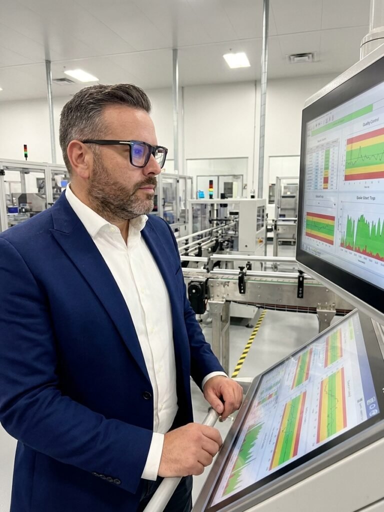
Statistical Process Control charts serve as an early warning system across all phases. A stable, in-control process maintains the flat failure rate of useful life. Drifting control chart data on critical dimensions—such as mould temperatures or torque values—often signals the onset of wear-out mechanisms in the production equipment itself.
Industry 4.0 technology accelerates this integration. IoT sensors, machine learning algorithms, and digital twins allow engineers to monitor degradation curves in real time. The fundamental physics of the bathtub curve remain unchanged, but modern tools provide visibility into failure mechanisms months before traditional warranty data would reveal a trend.
I have audited plants that capture massive volumes of sensor data but lack the engineering discipline to map it against the Weibull distribution. More data does not improve reliability. Applying the correct statistical model to that data and executing the resulting engineering decisions is what reduces warranty costs and drives system excellence.