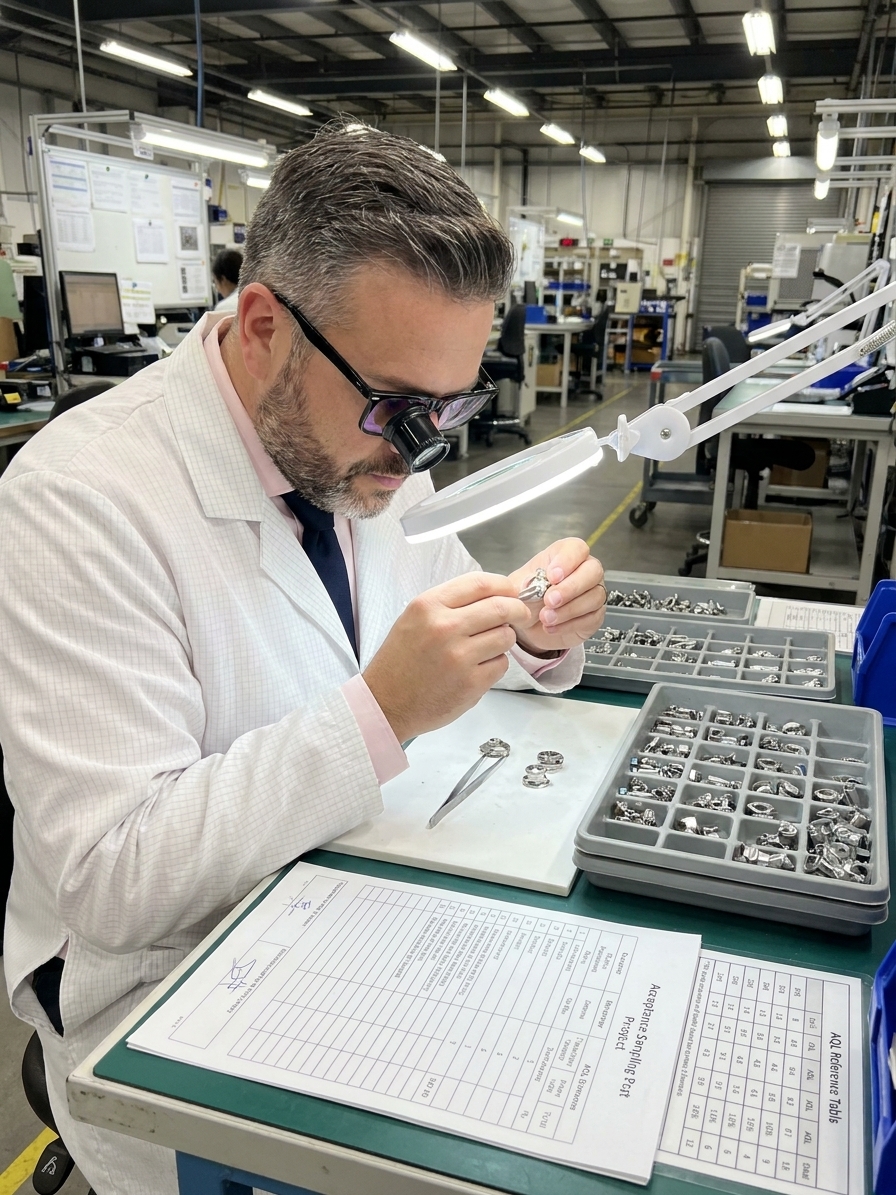
Every manufacturing organisation that ships product relies on the same fundamental mechanism: pull a sample, count the defects, compare to a table, and accept or reject the batch. It looks rigorous. The tables feature alpha-numeric codes that suggest deep statistical authority. In the hands of a practitioner who understands probability theory, acceptance sampling is a highly effective tool.
But that is rarely how the system is applied on the shop floor. Most organisations use acceptance sampling as a bureaucratic shield. They pull samples that are too small, apply criteria they do not understand, and make decisions disconnected from actual risk. They approve batches that should have been rejected, reject batches that were statistically fine, and wonder why customer complaints persist.
The result is a quality system that generates impressive documentation while providing negligible protection. The tables everyone trusts — ANSI/ASQ Z1.4 and ISO 2859-1, derived from the legacy MIL-STD-105E — have become a statistical costume. They allow organisations to pretend they control what they are shipping. To break this illusion, quality leaders must understand the mechanics of the Operating Characteristic curve.
The Core Mechanism: Probability, Not Guarantees
Acceptance sampling is a statistical method for making a binary decision about a population based on a fraction of that population. You define a sample size (n) and an acceptance number (c). You inspect n units. If you find c or fewer defects, you accept the lot. If you find more than c, you reject it. Everything else in the standard is just a systematised way of choosing n and c based on lot size and desired protection.
The foundational concept that most practitioners miss is that acceptance sampling does not tell you whether a lot is good or bad. It tells you the probability of accepting a lot at a given quality level. There is always a chance of accepting a defective lot (consumer's risk) and a chance of rejecting a conforming one (producer's risk). The entire discipline is about managing those probabilities, not eliminating them.
This misunderstanding creates a false sense of security across the supply chain. When a lot passes inspection, downstream departments treat it as factually defect-free. The stamp of approval overrides the statistical reality. The acceptance result is not a guarantee of zero defects; it is an inference with a known, quantifiable error rate that you have agreed to tolerate.
AQL Versus LTPD: The Risk Equation You Ignore
AQL stands for Acceptable Quality Limit. It is the worst tolerable process average that you, as the customer, are willing to accept as a routine outcome. An AQL of 1.0 percent means you are willing to accept lots where up to 1 percent of the units are defective. You are explicitly agreeing to tolerate that defect rate, not guaranteeing that the lot meets that threshold.
Most organisations treat AQL as a physical guarantee. They believe that inspecting to AQL 1.0 means the lot contains less than 1 percent defects. It does not. What it actually means is that if the lot is exactly 1 percent defective, the sampling plan will accept it approximately 95 percent of the time. The lot could easily be 2 or 3 percent defective and still pass inspection based on a small sample size.

Real consumer protection comes from a different metric: LTPD, or Lot Tolerance Percent Defective. This is the quality level you want to reject most of the time — typically with 90 percent probability. The gap between the AQL and the LTPD defines the discriminating power of your sampling plan. If you do not know your LTPD, you have no idea how many defective units you are actually shipping to your customers.
The Operating Characteristic Curve: The Hidden Reality
Every sampling plan has an Operating Characteristic (OC) curve. This graph plots the probability of accepting a lot against the actual, underlying defect rate of that lot. The steeper the curve, the more discriminating the plan. A perfect inspection (100 percent sorting) would be a vertical step function. Any sampling plan falls short of that ideal, and the OC curve shows you exactly how far short it falls.
I have walked into plants where the quality manager could recite AQL values from memory but had never plotted the OC curve for their own sampling plan. When we plotted it together, the result was always the same: shock. They realised their rigorous inspection program was catching maybe half the bad lots and letting the rest walk out the loading dock.
Anatomy of a Weak Sampling Plan
If your OC curve is shallow — which it will be if your sample size is small relative to your lot size — then there is a significant probability of accepting lots with defect rates far above your AQL. You might set AQL at 0.65 percent and still routinely accept lots at 3, 5, or even 10 percent defective. The mathematics do not lie. The data simply never gets shown to the people making the commercial decisions.
The Sample Size Trap and Special Inspection Levels
The most common error in acceptance sampling is using sample sizes that are far too small to provide meaningful discrimination. Organisations blindly follow AQL tables without considering that the tables provide different sample sizes based on inspection levels. The default Level II gives moderate protection. But many use special inspection levels (S-1 through S-4) for convenience, instantly trading away their statistical protection.
I once audited a manufacturer using Inspection Level S-2 for incoming inspection of critical components. They were pulling 5 units from lots of 5,000. When we plotted the OC curve, we found they had a 40 percent chance of accepting lots with 15 percent defects. The quality manager was stunned. He had been following the standard meticulously. He just had not understood what the standard actually meant.
Organisations also confuse sampling for accept/reject decisions with sampling for estimation. If you want to estimate the defect rate in a lot, you need a much larger sample than if you simply want to decide whether to accept or reject it. Many engineers feed data into their SPC system using sample sizes designed for acceptance decisions. The result is estimates with confidence intervals so wide they are statistically meaningless, presented in charts that look incredibly precise.
Switching Rules: The Feedback Loop Everyone Ignores
The ISO 2859-1 sampling system includes switching rules designed to dynamically adjust inspection rigor based on recent quality history. If a supplier's recent lots are good, you switch from normal to reduced inspection, saving cost. If they are bad, you switch to tightened inspection with larger samples and stricter criteria. If they stay bad, you discontinue acceptance altogether.
These switching rules are the feedback mechanism that makes the system adaptive. Without them, AQL inspection degrades into a static ritual. In practice, almost nobody follows the switching rules. The system requires meticulous record-keeping, continuous attention, and the willingness to disrupt production by changing the sampling plan. Most organisations simply pick a plan, write it into their procedure, and use it forever.
The Neglected ISO 2859-1 Switching Sequence
- 01Normal InspectionBaseline sample sizes and acceptance numbers applied to new suppliers.
- 02Tightened InspectionTriggered by 2 out of 5 consecutive lots rejected; demands lower AQL thresholds.
- 03DiscontinuationTriggered by 5 consecutive rejections under tightened rules; halts acceptance.
- 04Reduced InspectionAllowed after 10 consecutive accepted lots; slashes sample sizes to cut cost.
The consequences are entirely predictable. Suppliers whose quality has deteriorated keep getting inspected at the same static level they earned years prior. Lots that should trigger immediate tightened inspection sail through because nobody tracks the history. By the time the problem becomes visible in customer complaints or warranty claims, the damage is already done.
Double Sampling: Complexity Without Competence
The AQL system includes provisions for double and multiple sampling plans. You take an initial sample, and if the results are inconclusive, you take additional samples before making a final decision. In theory, these plans reduce the average sample size while maintaining the same statistical protection. In practice, they introduce profound operational risk.
Double sampling introduces the temptation to give the lot another chance. An operator pulls the first sample, finds too many defects, and instead of rejecting, takes a second sample hoping it will bring the average down. This is statistically invalid — the second sample size and combined acceptance numbers must be predetermined — but it is how operators often interpret the instruction.
Acceptance sampling sits at the bottom of the quality hierarchy. It is the last line of defence, not the first.
The result is a biased process that accepts more defective lots than the plan was designed to permit. Multiple sampling is even worse, requiring careful tracking of cumulative defects against shifting boundaries. If your organisation has not mastered single sampling — and most have not — implementing double or multiple sampling simply adds dangerous complexity to a system that is already failing at the basics.
The Strategic Fix: Prevention Over Detection
Acceptance sampling was designed for military procurement during World War II — a context where inspectors needed to make rapid decisions about massive shipments of munitions, and 100 percent inspection was practically impossible. It is a defensive measure, not a quality improvement tool. It does not prevent defects. It does not identify root causes. It sorts good lots from bad lots, imperfectly, after the defects have already been produced.
If your organisation relies on acceptance sampling as its primary quality control mechanism, you have effectively resigned yourself to catching defects rather than preventing them. The hierarchy of controls has been clear since Feigenbaum defined it: prevent first, control second, inspect last. When your team spends more time pulling samples than improving PFMEA and control plans, your priorities are exactly backward.
Plot the OC curves for every sampling plan you currently operate. Follow the ISO 2859-1 switching rules religiously. Align your AQL values with actual customer risk tolerance, not arbitrary defaults. And aggressively invest in prevention. Every hour spent stabilising a process at the source saves ten hours of downstream sorting. The ultimate goal is to make acceptance sampling entirely irrelevant to your operation.