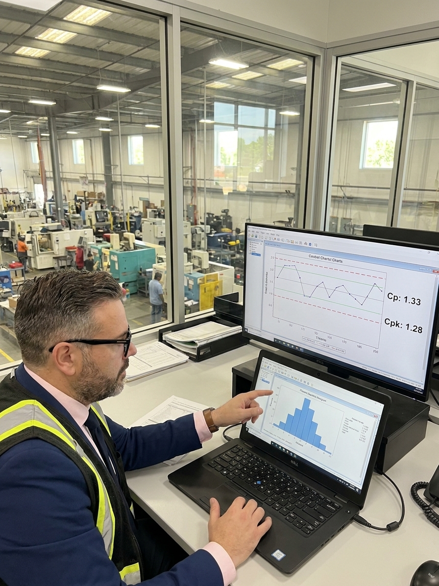
Cp and Cpk sit at the top of nearly every automotive and aerospace quality dashboard. Customers demand them in PPAP submissions, auditors check them against IATF 16949 and AS9100 requirements, and management uses them to gauge plant health. A Cpk of 1.33 acts as the universal threshold separating an approved process from one requiring containment.
Despite this reliance, process capability indices are among the most widely misused tools in manufacturing quality. They are simple arithmetic ratios treated as absolute truth. The calculations compress complex process behaviour into a single number, stripping away the context engineers need to diagnose problems.
These indices capture a snapshot dependent on statistical assumptions your process may not satisfy. They are calculated using data your measurement system may not have validated, presented with a precision your sample size cannot support. The gap between what these numbers indicate and what the floor is actually doing generates preventable defects.
The Mechanics of Cp and the Lie of Symmetry
Cp is the simplest capability index. It defines the ratio of your specification width to your process spread: Cp = (USL – LSL) / 6σ. A Cp of 1.0 means your ±3σ spread exactly fits the specification window. A Cp of 2.0 means your process spread is half the specification width, representing the Six Sigma benchmark.
The formula assumes your data is normally distributed, statistically stable, and accurately measured. If any assumption fails, the resulting number is fiction. The most dangerous failure is the lie of symmetry. Cp completely ignores process centering.
A process hugging the upper specification limit and a perfectly centered process will yield the exact same Cp if their spreads are identical. Cp reports potential capability, assuming you can hold the mean perfectly centered. It provides zero indication of what the process is producing right now.
I have audited plants where a quality manager presented a Cp of 1.67 on a critical dimension. The dashboard was green and the customer had signed off. An examination of the raw data revealed the process mean was shifted 2.5 standard deviations toward the upper limit. The process was theoretically capable and actively producing scrap.
Cpk, Centering, and the Minimum Function Mask
Cpk was developed to solve the centering problem. The formula calculates the minimum of two ratios: Cpk = min[(USL – μ) / 3σ, (μ – LSL) / 3σ]. It evaluates the distance from your process mean to the closest specification limit, divided by 3σ.
If your process is perfectly centered, Cp equals Cpk. As the mean drifts, Cpk drops. The mathematical difference between Cp and Cpk quantifies the capability lost to poor centering. This calculation is highly useful for identifying immediate drift, but it remains structurally incomplete.
Because Cpk is a minimum function, it only reports the worst-case side. It completely masks the headroom on the opposing specification limit. A process running dangerously close to the lower limit will display a terrible Cpk, hiding the fact that the upper side has enormous, unreported tolerance available.

More critically, Cpk is calculated from sample data. With a standard sample size of 30 consecutive parts, the estimate carries a confidence interval of roughly ±0.3. A reported Cpk of 1.33 could actually sit anywhere from 1.03 to 1.63, spanning the gap between capable and non-capable.
Standard Capability Thresholds and Risks
The Normality Assumption and Subgroup Manipulation
Every textbook on statistical process control dictates that data must be normally distributed for capability indices to hold. In real manufacturing, tool wear creates trends, material lot changes create shifts, and multi-stream processes create mixture distributions that look nothing like a bell curve.
When non-normal data feeds a standard capability formula, the indices break. Skewed distributions produce capability estimates wrong in unpredictable directions. Bimodal distributions from multi-cavity molds yield entirely meaningless indices because no single curve describes the physical reality.
Software offers Box-Cox transformations and non-parametric tolerance intervals to handle these realities. Yet, in my experience reviewing capability studies across aerospace and automotive suppliers, engineers skip these tools over 90% of the time. They apply the normal assumption, generate the number, and submit the report.
The standard deviation used in the denominator dictates the outcome. If you calculate σ from a month of daily measurements, between-shift variation inflates the spread, artificially deflating your capability. You spend capital chasing variation that is not inherent to the machine itself.
Conversely, calculating σ from five consecutive parts captured within minutes provides the most optimistic view possible. The resulting high capability index ignores material and environmental drift. The process looks world-class on paper while shipping non-conforming parts when the humidity changes.
How Sample Size and Specifications Distort Reality
Small sample sizes hide distribution shapes. A 10-part sample might yield a Cpk of 1.50, easily passing a customer mandate. Expanding that sample to 1,000 parts from the same process often reveals a slight right tail. The actual defect rate can jump from the assumed 3.4 parts per million to 50 parts per million.
This invisible tail generates field failures. You must report capability indices with a lower confidence bound, known as Cpk-L. If the lower 95% confidence bound sits below your threshold, you lack the statistical evidence to claim capability. This practice remains standard in statistics and rare on the shop floor.
A capability index is a description of a process that does not exist if the process is changing while you measure it.
Even with perfect mathematics, capability indices are ratios comparing your process to your specifications. If the specifications are wrong, the index measures performance against a target that carries no functional value. I routinely find tolerances carried forward from 30-year-old drawings, tied to outdated machining capabilities for products redesigned multiple times.
Engineers also specify tolerances too wide, aiming to guarantee a high Cpk on the dashboard. The process reports a Cpk of 2.0, but the functional performance of the final assembly suffers because the loose tolerance allows excessive play. The metric looks perfect while the product fails.
Three Failure Modes in Capability Reporting
Pre-launch inflation occurs when a quality team runs the capability study during a pilot using hand-picked material and the best operator. The study yields a Cpk of 1.80, securing customer sign-off. Once full production starts across three shifts and varying ambient conditions, the Cpk drops to 1.15 within weeks.
The cherry-picked subgroup involves a supplier reporting a Cpk of 1.50 on a dimension linked to field failures. An audit reveals the study covered 50 parts from the single best run of the month. The true capability across all production runs sits at 0.95. The supplier optimised the data rather than reporting reality.
Silent drift happens when a process maintains a Cpk above 1.33 for two years based on rolling 30-point calculations. The data looks stable month to month. Plotting 24 months on a single control chart reveals a steady 0.2σ drift per month. The process has drifted 4.8σ over two years, pushing tail-end parts out of specification.
Dashboard Metrics Versus Process Reality
What teams report
- A single Cpk value of 1.33 from 30 parts
- Normal distribution assumed without testing
- Total compliance with customer PPAP mandates
- Process stability based on point estimates
What actually exists
- A confidence interval spanning non-capable limits
- Skewed data from multi-cavity mold mixtures
- Optimistic calculations from pilot run conditions
- Slow mean drift hidden by rolling data windows
Building a Reliable Capability Analysis Process
Always verify normality before running indices. If the Anderson-Darling test fails, use Box-Cox transformations or distribution-specific capability models. Accompany every index with a control chart. If the process is not in statistical control, the capability index describes a process that currently does not exist.
Decompose your variation using nested ANOVA or variance components analysis. Break the total sigma down into within-part, between-batch, between-shift, and between-machine variation. This decomposition tells engineering exactly where to target improvement capital instead of guessing at a broad number.
Enforce the use of lower confidence bounds on all internal and customer-facing reports. Mandate that any submission meeting customer thresholds must also pass MSA requirements, specifically confirming that the gauge R&R contributes less than 10% of the observed variation.
Challenge specifications during APQP reviews. Demand to know the functional basis for every tolerance. Releasing a drawing without understanding the geometric dimensioning and tolerancing impact forces manufacturing to chase arbitrary targets, distorting the capability data from day one.