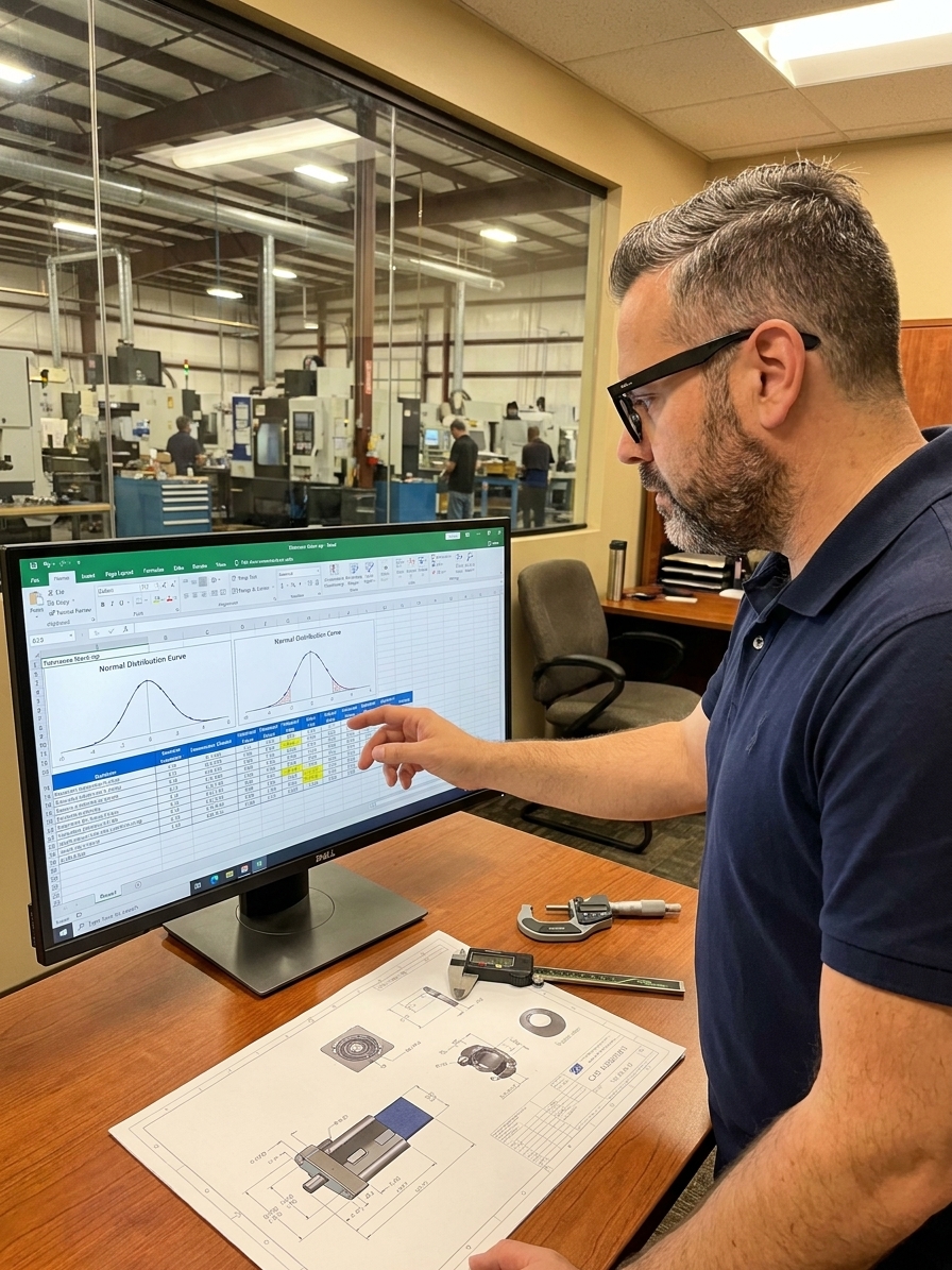
Scaling a product from a single pilot line to three manufacturing sites is where tolerance analysis breaks. The drawings, the GD&T, and the validated stack-up models remain unchanged. The physical hardware, however, suddenly exhibits assembly failures that the development engineers never witnessed in the prototype phase.
The cause is not poor workmanship at the new locations. The analytical models that justified the original drawing release were calibrated for a single, highly controlled machine. When production scales across multiple facilities, diverse machine tools, fixture variations, and localized environmental conditions introduce entirely new variables into the stack-up.
Across two decades implementing IATF 16949 and AS9100 quality systems, I have audited multi-site rollouts where unmanaged tolerance drift consumed the entire projected profit margin. Organizations treat tolerance analysis as a design milestone rather than a living manufacturing control. When production volume and supplier diversity increase, that static approach guarantees expensive field failures and internal scrap.
How Multi-Site Production Breaks RSS Assumptions
Root Sum Square (RSS) analysis is the standard method for calculating likely assembly variation. It takes the root sum square of individual component standard deviations. The mathematics are sound, but they rest on rigid assumptions: component dimensions must follow a normal distribution, remain centred on the nominal, and be statistically independent.
A single high-precision CNC machine in a controlled pilot cell will likely meet these criteria. The process is stable, the tool wear is predictable, and the operator is highly trained. The RSS calculation accurately predicts assembly yield because the physical process actually matches the mathematical model. The resulting Cp and Cpk values reflect a controlled, singular environment.
Transferring that same part to three different tier-one suppliers shatters these assumptions. Supplier A machines the part on a horizontal mill; Supplier B uses a vertical machining centre. The process distributions are no longer normal or identical. Tool wear patterns differ. Sudden setup variation shifts the process mean between batches, rendering the original Cpk 1.33 baseline obsolete.
When these distinct, non-normal distributions converge at the final assembly plant, the statistical independence vanishes. A casting datum surface that is consistently off-nominal at Supplier C shifts every subsequent dimension referenced from it. The RSS model predicts 99.9% yield, but the physical multi-site assembly line struggles to achieve 97%.
The Cost of Unmanaged Complexity at Volume
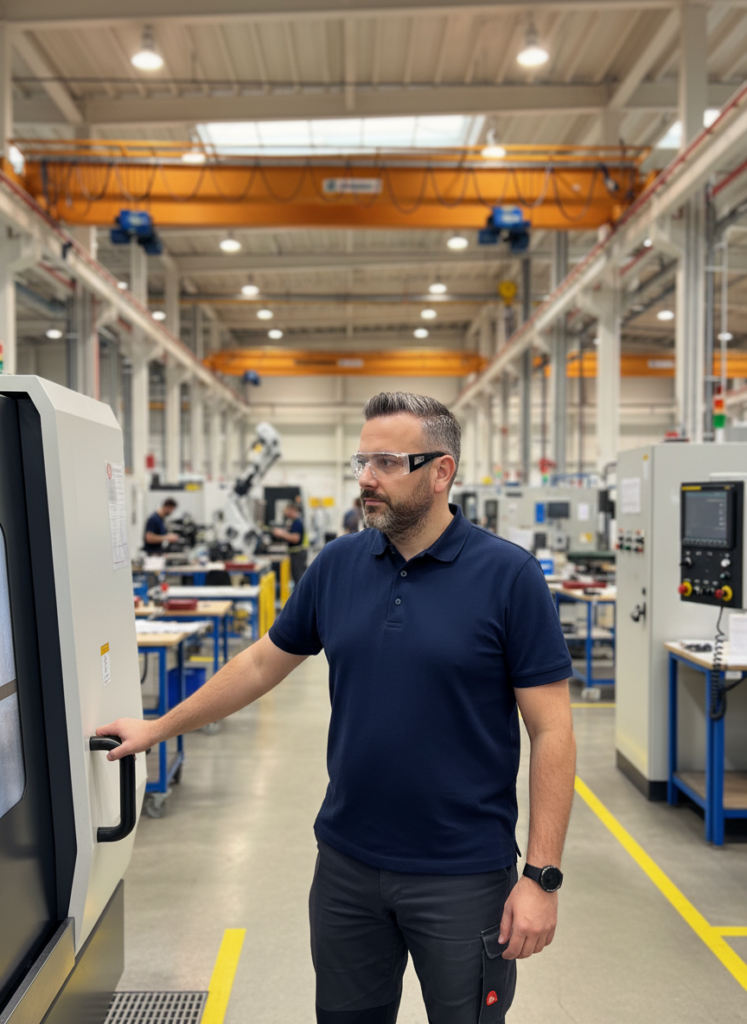
As product mix increases, the volume of tolerance data expands exponentially. A single automotive sub-assembly might involve fifty dimensions across five suppliers. If the organization relies on worst-case arithmetic to manage this complexity, the stack-up variation forces engineers to tighten component tolerances far beyond functional requirements.
Over-engineering at volume is a hidden profitability drain. Forcing a supplier to hold a non-critical dimension to ±0.02 mm because the worst-case calculation demanded it drives up tooling costs, reduces tool life, and slows cycle times. When multiplied across 100,000 units, the cost of guarding against a mathematical impossibility becomes catastrophic.
The alternative is allowing looser tolerances without updating the analytical model. When engineering teams fail to correlate the looser supplier tolerances with the final assembly yield, scrap rates at the OEM plant spike. The gap between the planned mathematics and the physical hardware is paid for in sort operations, rework lines, and expedited freight.
Process Capability Thresholds for Scaled Tolerance Models
Deploying Monte Carlo Across a Supplier Network
When production scales, the analytical limitations of RSS demand a more robust tool. Monte Carlo simulation replaces the normal distribution assumption with brute-force computational power. Instead of assuming statistical independence, the simulation is fed the actual measured distributions from every supplier and every machine tool in the network.
The advantage of Monte Carlo is absolute flexibility. It accurately models non-normal distributions, correlated datums, shifted process means, and complex geometric tolerancing scenarios required under AS9100 or IATF 16949. It provides a realistic yield prediction for a multi-facility assembly by acknowledging the physical reality of diverse manufacturing environments.
The barrier to deploying Monte Carlo at scale is data infrastructure. The simulation requires knowing the actual mean, standard deviation, skewness, and kurtosis of each manufacturing step. If the supplier network does not maintain high-resolution statistical process control (SPC) data, the simulation degrades into guessing distributions instead of measuring them.
A Monte Carlo simulation fed with estimated inputs is not a valid engineering analysis. It produces highly precise numbers that are systematically wrong. Before deploying advanced statistical models across a multi-site network, the organization must first ensure that SPC data collection is standardized, automated, and mandatory across every node in the manufacturing chain.
Deploying Tolerance Models Across Multiple Sites
- 01Capture pilot baselinesRecord high-resolution SPC data from the original equipment to establish the true process distribution.
- 02Map new site variationsIdentify machine tool differences, fixture constraints, and environmental factors at the receiving facilities.
- 03Run cross-site Monte CarloInput the actual measured distributions from the new sites into a correlated simulation model.
- 04Validate physical yieldMeasure a statistically significant sample of pilot assemblies from the new sites and compare against predictions.
- 05Lock the PDM modelTie the validated analysis directly to the CAD model and mandate updates whenever process drift is detected.
Engineering Governance for Tolerance Lifecycles
The core organizational failure mode in multi-site production is treating tolerance analysis as a static checkbox. A design engineer validates the stack-up during development, files the document, and moves to the next project. The analysis lives in a spreadsheet, disconnected from the physical manufacturing reality it is supposed to govern.
When a supplier changes a tooling process, or when a new site alters the manufacturing routing, nobody updates the analysis. The drawing remains released at tolerances that no longer reflect the actual process capability. This disconnect guarantees that the quality organization will spend months chasing variation through reactive 8D investigations instead of preventing it through engineering governance.
Tolerance analysis is a living engineering document, not a milestone deliverable. If it sits in a file, it is already obsolete.
Building functional governance requires embedding the tolerance model inside the product data management (PDM) system. The analysis must be tied directly to the CAD geometry. When an engineering change order alters a tolerance, or when a supplier change alters the process distribution, the PDM system must mandate a tolerance review before the change is approved.
Single-point ownership is critical. Assign one engineer responsible for the integrity of each major stack-up across the entire product lifecycle. This engineer ensures that when the production volume doubles or the supplier base expands, the statistical models are re-evaluated with live SPC data.
Validation Studies and SPC Data Integration
No analytical method works without physical validation at the receiving plant. Whatever the Monte Carlo simulation or RSS calculation predicts, the only way to verify a scaled production model is to measure actual assemblies coming off the new lines. This physical validation step is systematically ignored during rapid scaling.
Before a product moves from pilot to full multi-site production, the quality organization must measure a statistically significant sample of physical assemblies. If the predicted yield does not match the physical measurements, the underlying statistical assumptions must be corrected before authorizing the scale-up. This validation must be a mandatory gate in the APQP or PPAP process.
The quality team must maintain a live database of process capability for each manufacturing operation and each supplier. This central repository replaces the default tolerance-divided-by-three assumption with real, measured standard deviations. It allows the engineering team to see exactly when a process at a specific facility is drifting toward failure.
When field failures or in-process defects trace back to tolerance issues, the resulting 8D investigation must force an update to the central tolerance model. This closes the loop. It transforms tolerance management from a theoretical engineering calculation into a robust, data-driven operational discipline that scales safely with the business.