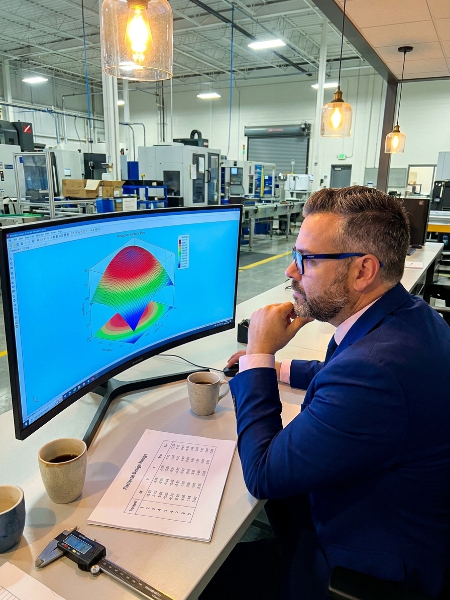
When a structured Design of Experiments (DOE) initiative fails to deliver actionable results, the mathematics are rarely to blame. Modern statistical software platforms like Minitab and JMP generate flawless experimental matrices and Analysis of Variance (ANOVA) outputs instantly. The failure almost always occurs upstream, during the unstructured diagnostic phase where engineers decide what to test.
Across two decades implementing IATF 16949 and AS9100 systems in automotive and aerospace plants, I have reviewed countless failed experimental designs. The recurring theme is a rush to execute a fractional factorial matrix before understanding the physical process constraints. Teams treat DOE as a mathematical search engine rather than a validation tool for process physics. They feed the matrix poorly defined variables and receive statistically significant nonsense in return.
A successful DOE requires a rigorous diagnostic phase to prepare the process environment. This preparation involves mapping the physical failure dynamics, verifying the measurement infrastructure, and defining factor boundaries that reflect mechanical reality. Skipping this diagnostic work guarantees that the experimental runs will generate expensive confusion rather than actionable process knowledge.
Identifying the Physical Failure Mechanism First
Engineers frequently select experimental factors based on machine parameter menus rather than physical failure analysis. A screen listing injection speed, holding pressure, and melt temperature invites operators to test all three independently. But if the actual failure mechanism is residual thermal stress, the dominant variable might be mold cooling channel geometry, which is never presented as an adjustable setpoint on the controller.
Effective experimental design starts with a rigorous Physics of Failure analysis. You must trace the defect back to its mechanical, chemical, or electrical root cause before opening the statistics software. If you are investigating a porosity defect in a casting process, you must understand whether the gas is being entrapped mechanically during die fill or precipitating chemically during solidification. These two mechanisms require entirely different experimental factors.
Cross-functional teams must map the entire value stream to identify these true driving factors. A Process FMEA (PFMEA) provides the ideal foundation for this diagnostic work. By linking the failure mode to a specific physical mechanism, you ensure the subsequent experimental matrix tests the variables that actually drive the defect, rather than the variables that happen to be easiest to adjust on the production floor.
If the vital physical variables cannot be controlled or measured during the experiment, you must redesign the test apparatus or abandon the design. Testing a proxy variable that is easy to adjust but disconnected from the physics wastes production capacity. The diagnostic phase exists precisely to prevent this misallocation of manufacturing resources.

Validating Measurement Integrity Before Testing
Measurement System Analysis (MSA) is the most critical prerequisite for any experimental design. If the gauge cannot reliably distinguish between good and bad parts, the ANOVA will calculate the variance of the measurement error rather than the variance of the process. This produces confidence intervals that look mathematically rigorous but describe the gauge, not the manufacturing process.
Conduct a formal Gauge R&R (Repeatability and Reproducibility) study on every measurement system used to capture the experimental response. The standard automotive threshold demands total Gauge R&R below ten percent of the study variation, though highly capable processes may require even tighter discrimination. If the gauge consumes thirty percent of the tolerance, your DOE is essentially measuring measurement noise.
Attribute measurement systems present a more deceptive trap. When operators pass or fail parts visually, the inspection process itself acts as a filter. A DOE designed to reduce visual defects like flash or sink marks fails when the visual inspection cannot reliably separate a true defect from acceptable process variation. An Attribute Agreement Analysis must quantify inspector bias and effectiveness before any experimental runs begin.
Calibration records are not a substitute for MSA. A torque wrench calibrated to traceable standards last week can still produce unacceptable measurement variation in the hands of a fatigued operator on the night shift. The diagnostic phase must verify how the measurement system performs under actual production conditions, not how it performs on a calibration bench.
Defining Factor Boundaries Against Process Drift
Setting factor ranges is the most subjective and error-prone step in experimental design. Engineers routinely set the high and low levels of a factor based on the machine's documented operating limits. This approach ignores the reality of ambient drift and shift-to-shift variation. The experimental range must be wide enough to trigger a measurable response, yet narrow enough to remain within the engineering process capability.
If you set the difference between the high and low settings smaller than the natural process variation, the experiment will fail to detect the main effect. The signal will be lost in the operational noise. Conversely, pushing the boundaries to the point where the process produces pure scrap teaches you nothing about optimization. The math will simply confirm where the process breaks, which you already knew.
I have audited manufacturing plants where expensive experimental runs were wasted because the ambient temperature shifted between the morning and afternoon trials. This systematic drift confounded the primary factor, rendering the statistical model invalid. The diagnostic phase must identify these potential noise variables and account for them through blocking, randomization, or environmental control.
DOE Process Readiness Pipeline
- 011. Physics MappingTrace defect to mechanical root cause via PFMEA.
- 022. MSA ValidationConfirm gauge discrimination via Gauge R&R.
- 033. Range SettingAdjust boundaries wider than natural noise, narrower than scrap limits.
- 044. RandomizationInsulate main effects from ambient time-shifted drift.
Isolating Variables in Batch Versus Continuous Processes
The diagnostic approach changes fundamentally depending on whether you are running a batch process or a continuous flow. In aerospace composite curing, an autoclave run represents a massive capital expenditure. Running a sixteen-run full factorial design is economically impossible when each cure cycle takes eight hours. The diagnostic focus shifts toward Augmented D-Optimal designs that extract maximum information from a heavily restricted number of physical runs.
Continuous processes, such as extrusion or chemical vapour deposition, allow for more experimental runs but suffer heavily from autocorrelation. Adjusting a screw speed parameter takes time to propagate through the system and stabilize. If you take a sample before the system reaches steady state, you are recording transient noise rather than the true process response.
These constraints demand different diagnostic strategies. In aerospace, I have seen teams successfully use historical production data to build initial response models, validating them with a sparse handful of targeted confirmation runs. In continuous automotive extrusion, engineers must calculate the physical residence time of the material and build that stabilization delay directly into the experimental run sheet.
Recognizing the physical constraints of the production system before designing the experiment prevents statistical blindness. A perfectly balanced orthogonal matrix is useless if the production line physically cannot execute the randomized run order without compromising the material stability.
Structuring the Confirmation Run Strategy
A DOE outputs a mathematical prediction, not a manufacturing guarantee. Once the response surface methodology identifies the optimal process settings, the diagnostic work resumes. The confirmation phase verifies whether the mathematical model actually holds true on the physical shop floor under standard operating conditions.
Too many organizations treat the software's predicted optimum as the final answer. They update the Standard Operating Procedure (SOP) and walk away. A rigorous confirmation strategy requires running the predicted optimal settings alongside the current baseline settings in a randomized, blind test. If the optimized settings do not demonstrate a statistically significant improvement over the baseline, the model is incomplete.
An incomplete model usually means a significant interaction was missed during the initial screening phase. Perhaps a humidity variable was assumed constant during the test but fluctuated wildly in production. The confirmation run exposes these hidden dependencies. If the confirmation fails, you must return to the diagnostic phase rather than forcing the new settings into production.
DOE forces you to test the conditional dependencies that process intuition cannot imagine.
The confirmation phase is also where you establish long-term statistical control. Transitioning from the experimental optimum to a validated Cpk target requires running a production capability study over an extended period. This final diagnostic step bridges the gap between statistical experimentation and the daily reality of sustaining manufacturing quality.
Translating Statistics Into Process Control
The final objective of a DOE is not an academic paper; it is a robust update to the PFMEA and the Control Plan. The mathematical model generated by the experiment must be translated into operational language that operators and frontline supervisors can execute without needing to understand the underlying matrix algebra.
Every significant factor identified in the experiment must be paired with a specific control mechanism and a reaction plan. If the DOE identifies incoming material temperature as a critical variable, the Control Plan must specify how to measure it, what the acceptable range is, and exactly what adjustment the operator must make if it drifts outside that range.
Variables that proved insignificant during the experiment offer an equally valuable diagnostic benefit. If the screening design proves that ambient humidity has no measurable effect on the defect within the tested range, you can safely remove it from the daily quality tracking logs. This reduces operator workload and focuses quality attention on the mechanical variables that actually drive the process response.
The Hierarchy of Process Knowledge
- Mathematical ModelANOVA and response surfaces defining variable interactions.
- Control Plan UpdateSOPs detailing acceptable ranges and operator adjustments.
- PFMEA RevisionUpdated risk priority numbers reflecting validated variables.
- Sustained CapabilityLocked Cpk targets secured against main effects and interactions.
A manufacturing process is a physical system governed by interacting variables, not a list of independent machine settings. Building a sustainable DOE capability means training engineers to diagnose the physics before applying the statistics. When the diagnostic framework is respected, structured experimentation ceases to be an academic exercise and becomes the foundation of predictable manufacturing quality.