Cp, Cpk, Pp, Ppk: Why Short-Term Capability Hides Long-Term Failure

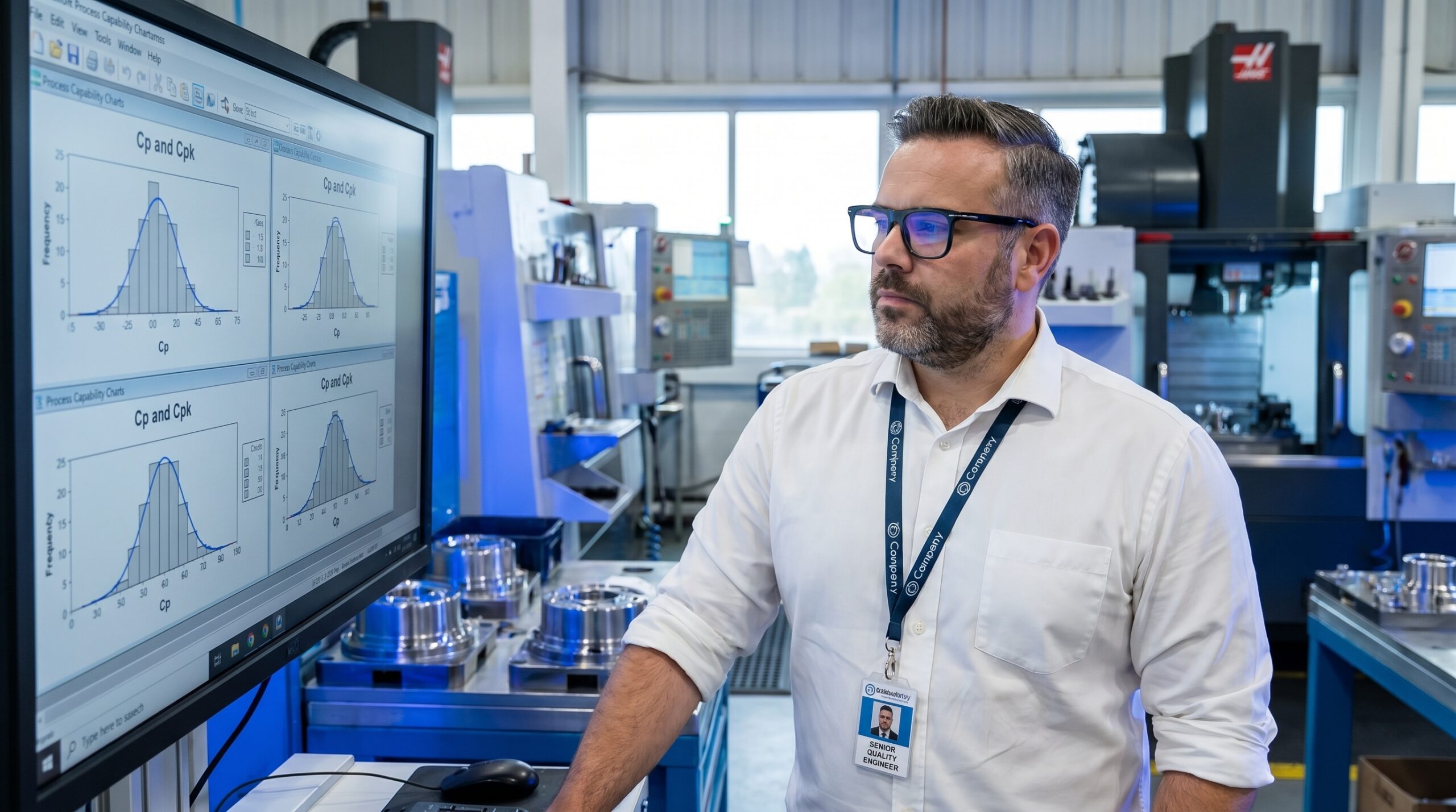
A quality engineer calls, frustrated that a customer rejected an entire shipment despite the plant reporting a stellar Cpk of 1.33. This scenario plays out across automotive and aerospace supply chains every month. Someone measures short-term capability, presents a beautiful index, and then acts surprised when long-term production reality looks entirely different.

Process capability is the mathematical ratio between what your process actually does and what the customer specification demands. The customer defines the upper and lower specification limits (USL, LSL). Your process generates its own mean and variation. If your process variation is narrow relative to the specification width, the process is deemed capable.

The critical failure is assuming process variation is a single, static value. It is not. Short-term variation captures the process under laboratory conditions. Long-term variation captures the process in the real world. Confusing the two guarantees that your capability reports will mislead your management and your customers.

Short-Term Variation: The Laboratory Condition

Short-term capability (Cp, Cpk) measures how the process behaves when everything is perfectly set up. This means material from a single homogeneous batch, an experienced operator at the controls, a freshly calibrated machine, and optimal ambient temperature. It represents your process potential.

You typically measure 30 to 50 consecutive parts in a short time frame. You calculate Cp and Cpk using the within-subgroup standard deviation (σ_within). This isolates the inherent machine and tooling variation. You will often get impressive numbers, easily clearing the IATF 16949 expectations for initial process studies.

The trap is that this variation metric deliberately excludes external noise. It does not account for tool wear, material lot changes, shift handovers, or hydraulic pressure drops. It tells you what your equipment can do in isolation, not what it will do over a six-month production run.

Long-Term Variation: The Real World

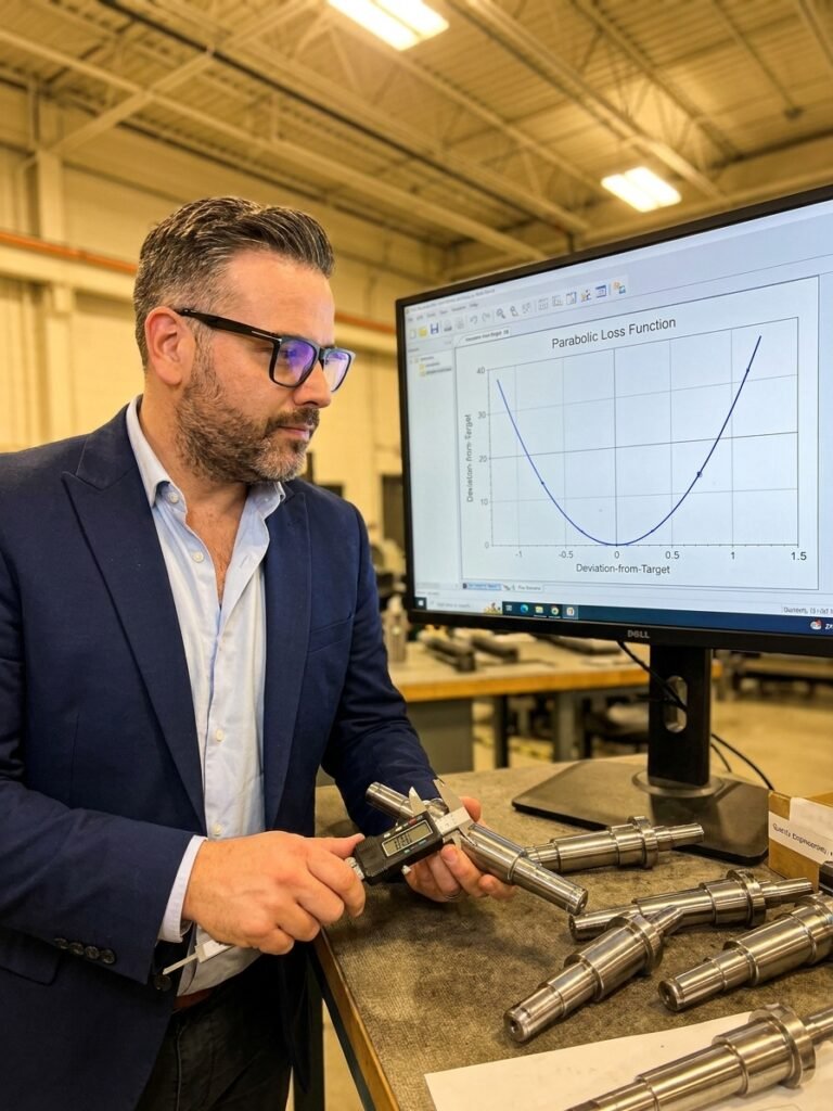
Long-term capability (Pp, Ppk) measures what happens when the process runs for weeks or months. It accounts for reality: a new vendor for raw material, a less experienced operator on the night shift, a tool nearing the end of its lifecycle, and ambient humidity changes.

These performance indices use the overall standard deviation (σ_overall). This metric includes both the within-subgroup variation and the between-subgroup variation. Consequently, it is almost always larger than the short-term variation. When a short-term Cpk of 1.33 is recalculated using long-term data, it frequently drops to a Ppk of 0.89.

A Ppk below 1.0 means the process is producing non-conforming parts. The customer does not experience your pristine short-term laboratory data. They experience your long-term performance, and if that performance falls outside their specification limits, they will reject the shipment.

The Mechanics of Process Drift

When reviewing SPC control charts for rejected lots, the process often appears statistically stable. There are no obvious special causes or sudden spikes. However, the data reveals a systematic drift across the production timeline.

A machine might produce parts 0.02 mm higher every Monday after a cold weekend start. A routine tool change might shift the mean by 0.015 mm. A new raw material lot might add another 0.01 mm of variance. Individually, these shifts are invisible in short-term studies. Accumulated over weeks, they increase overall variability by 30 to 40 percent.

This accumulation is the physical manifestation of the gap between Cp and Pp. The short-term study captured the machine cutting steel. The long-term data captured the reality of the factory floor operating through seasons, shifts, and supply chain variables.

Standard Capability Thresholds

1.00Marginal limitProcess consumes the entire tolerance. Any drift causes defects.

1.33Automotive baselineMinimum standard for serial production in IATF 16949 environments.

1.67Critical characteristicStandard safety net for high-risk or customer-specific safety features.

2.00Six SigmaExceptional performance providing massive long-term drift buffer.

The 1.5 Sigma Shift and Centring

In the early days of Six Sigma, Motorola established the convention that long-term variation typically exceeds short-term variation by 1.5 sigma. This was an empirical observation, not a law of physics. The actual shift depends entirely on how well you control your inputs.

In tightly controlled aerospace machining, the shift might be 0.8 sigma. In a high-volume automotive stamping plant with high operator involvement, it might reach 2.0 sigma. You must measure your own data to understand the true gap between your Cp and Pp.

Centring further complicates the picture. Cp and Pp measure potential spread, ignoring where the mean sits. Cpk and Ppk factor in centring relative to the specification limits. Operators often deliberately set the process toward the 'safer' side of a unilateral tolerance, inadvertently reducing the actual safety margin and lowering the Cpk.

Cp tells you what the machine could do; Ppk tells you what the factory actually delivers.

A Practitioner's Method for Capability Assessment

Over twenty years of implementing IATF 16949 and AS9100 systems, I have developed a rigid sequence for evaluating capability. Skipping the first step is the most common reason quality teams chase ghosts instead of solving variation.

You must verify statistical stability before calculating any index. If the control chart shows special causes, capability indices are mathematically invalid. You are calculating the average speed of a car that is randomly crashing and stalling. Bring the process under statistical control first.

Once stable, run your short-term study. Then, collect at least 30 days of continuous serial production data to calculate long-term performance. Compare the two. If the gap between Cpk and Ppk exceeds 20 percent, you have excessive external variation. You must launch an investigation into material lots, tooling wear, and ambient factors.

Correct Sequence for Process Capability Evaluation

1. 01Verify StabilityReview SPC charts for special causes. Do not proceed until the process is in control.
2. 02Short-Term StudyMeasure 30-50 consecutive parts to determine Cp and Cpk potential.
3. 03Long-Term StudyCollect 30 days of production data to calculate Pp and Ppk.
4. 04Gap AnalysisCompare Cpk to Ppk. A gap over 20% demands investigation of external variation sources.

Eliminating the Root Causes of Long-Term Variation

Mapping the sources of long-term variation leads to concrete countermeasures. We implemented a standardised start-up protocol for weekend cold stops, adding a warm-up cycle to eliminate Monday morning drift. We tied tool replacement to SPC trend triggers rather than rigid piece counts, catching wear before it shifted the mean.

We also instituted a rapid incoming inspection for every new material lot. This was not a full PPAP, but a targeted five-piece verification to ensure the raw material variance stayed within the established tolerance band.

Within three months, these actions raised the Ppk from 0.89 to 1.33. More importantly, the gap between Cpk and Ppk closed to under 10 percent. The short-term potential and the long-term reality were finally aligned. That alignment is the true hallmark of a capable, controlled manufacturing process.