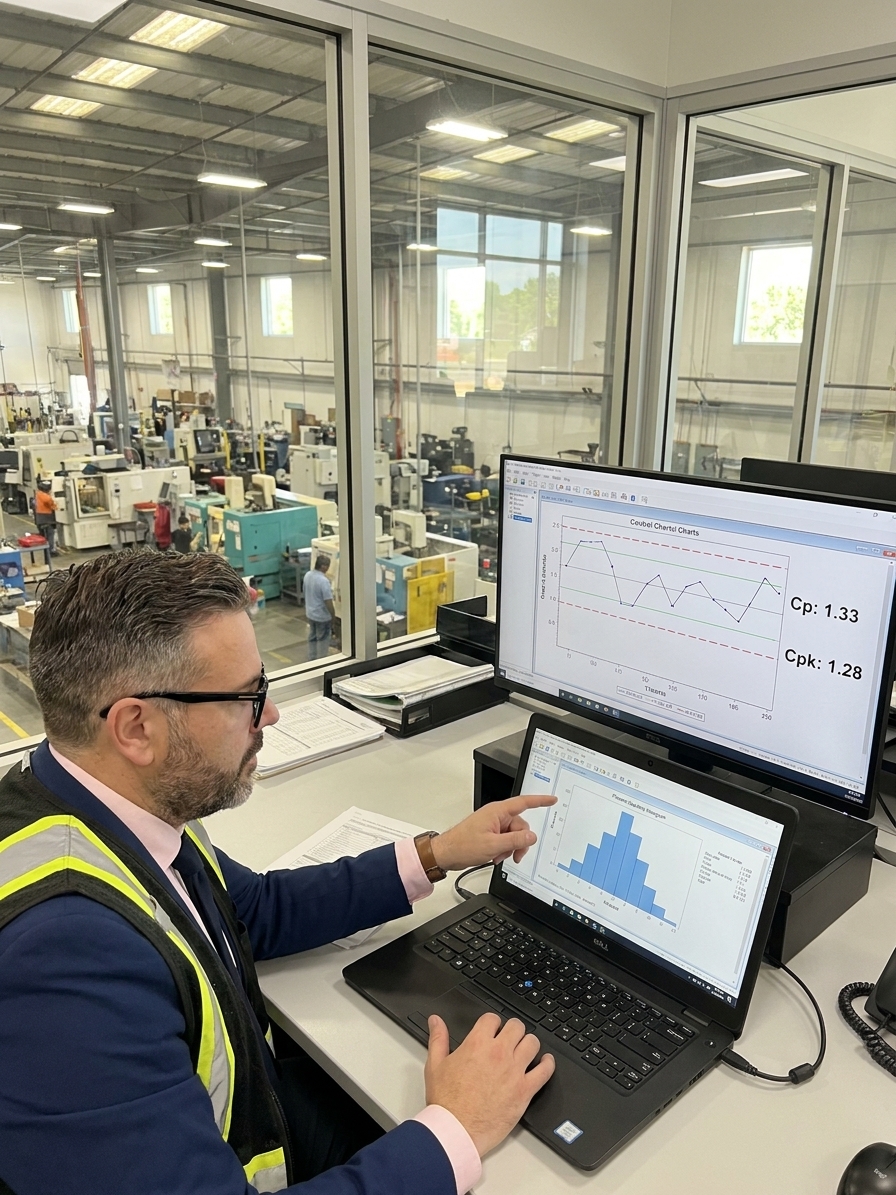
You’ve seen them on every quality dashboard. Cp. Cpk. Two little
numbers sitting side by side, one usually higher than the other, both
printed in green or red depending on whether they cross the magic
threshold of 1.33. Your management loves them. Your customers demand
them. Your auditors check them. And your engineers calculate them —
often incorrectly, usually without context, and almost always without
understanding what they actually mean.
Process capability indices are among the most widely used and widely
misunderstood tools in manufacturing quality. They are simple arithmetic
ratios that pretend to capture the entire relationship between your
process and your specifications. They don’t. They capture a snapshot — a
moment frozen in time, dependent on assumptions your process may not
satisfy, calculated from data your measurement system may not have
validated, and presented with a precision your sample size does not
support.
This article is about what Cp and Cpk actually tell you, what they
don’t, and why the gap between those two things has been the source of
more false confidence — and more preventable defects — than almost any
other metric in quality management.
What Cp Actually Measures
Cp is the simplest process capability index. It’s the ratio of your
specification width to your process spread:
Cp = (USL − LSL) / 6σ
Where USL is your upper specification limit, LSL is your lower
specification limit, and σ is your process standard deviation. A Cp of
1.0 means your process spread (±3σ) exactly fits your specification
window. A Cp of 1.33 means you have some room. A Cp of 2.0 means your
process spread is half your specification width — the holy grail of Six
Sigma.
Here’s what Cp assumes:
- Your process is normally distributed.
- Your process is in statistical control.
- Your data represents the actual process variation.
- Your specification limits are correct and meaningful.
If any one of these assumptions is wrong — and in real manufacturing,
at least one usually is — your Cp number is fiction. Not approximate.
Not conservative. Fiction.
The biggest lie Cp tells is the lie of symmetry. Cp doesn’t care
where your process is centered. A process hugging the upper
specification limit and a process sitting dead center between both
limits get the same Cp if they have the same spread. Cp tells you about
potential — what your process could achieve if it were perfectly
centered. It tells you nothing about what your process is actually doing
right now.
I’ve walked into plants where the quality manager proudly showed me a
Cp of 1.67 on a critical dimension. Green on the dashboard.
Customer-approved. Then I looked at the data: the process mean was
shifted 2.5 standard deviations toward the upper limit. The process was
capable in theory and scrap-producing in practice. The Cp number was
technically correct. The confidence it inspired was entirely wrong.
What Cpk Adds — and
What It Still Misses
Cpk was created to solve the centering problem. It accounts for where
your process actually sits relative to the specification limits:
Cpk = min[(USL − μ) / 3σ, (μ − LSL) / 3σ]
Where μ is your process mean. Cpk takes the worst-case side —
whichever specification limit is closer to your process average — and
reports capability based on that side alone. If your process is
perfectly centered, Cp equals Cpk. If your process is shifted, Cpk drops
below Cp. The difference between them tells you how much centering
you’ve lost.
This is useful. It’s also incomplete.
Cpk still assumes normality. Cpk still assumes statistical control.
Cpk still assumes your measurement system is adequate. And Cpk
introduces a new problem: because it’s a minimum of two ratios, it can
mask what’s happening on the other side. A process sitting right at the
lower specification limit with virtually no room on that side will show
a terrible Cpk — but the upper side might have enormous room that you’ll
never see reported in that single number.
More importantly, Cpk is calculated from sample data. The sample mean
and sample standard deviation are estimates, not parameters. With 30
data points — a common sample size — your estimate of Cpk has a
confidence interval roughly ±0.3 wide. That means a reported Cpk of 1.33
could actually be anywhere from 1.03 to 1.63. One side of that range
means your process is capable. The other side means it isn’t. And you’re
making shipping decisions based on a point estimate that spans both
realities.
The Normality
Assumption: The Elephant in the Room
Every textbook on process capability includes a caveat: “The process
must be normally distributed for these indices to be meaningful.” Every
practitioner nods. Almost nobody checks.
In practice, manufacturing processes deviate from normality
constantly. Tool wear creates trends. Material lot changes create
shifts. Gage resolution creates discrete distributions. Rework
operations create truncated distributions. Multi-stream processes
(multiple cavities, multiple machines, multiple operators) create
mixture distributions that look nothing like a bell curve.
When you feed non-normal data into a normal-based capability formula,
the result depends on how the data deviates. Heavy-tailed distributions
(more extreme values than normal) produce σ estimates that are too
large, making your capability index too small — conservative, but
misleading. Skewed distributions produce capability indices that are
wrong in unpredictable directions. Bimodal distributions — common when
two machines feed the same process step — produce capability indices
that are essentially meaningless because no single distribution
describes the data.
There are methods for handling non-normal data: transformations
(Box-Cox, Johnson), non-parametric tolerance intervals,
distribution-specific capability indices. These exist. They’re
documented. They’re implemented in every major statistical software
package. And they are used in perhaps 5% of the capability studies I’ve
reviewed in 25 years of practice. The other 95%? Normal assumption, plow
ahead, report the number, move on.
The
Subgroup Problem: How You Sample Changes What You See
The standard deviation in the capability formula is supposed to
represent your process’s inherent, common-cause variation. That’s the
variation you’d see if you measured consecutive parts under identical
conditions — the irreducible noise of your process.
In practice, people calculate σ from whatever data they have. A month
of daily measurements? That includes between-day variation, material
variation, operator variation, and environmental variation — all piled
on top of inherent process variation. The resulting σ is inflated. The
resulting Cp and Cpk are deflated. You think your process is worse than
it is, and you spend money chasing variation that isn’t inherent to the
process at all.
Conversely, some people calculate σ from a subgroup of 5 consecutive
parts measured within minutes of each other. That captures only
within-subgroup variation — the most optimistic possible view. The
resulting σ is too small. The resulting capability indices are too high.
You think your process is better than it is, and you ship parts that
drift out of specification when the shift changes, the temperature
drops, or a new material lot arrives.
The right answer depends on what you’re trying to communicate. If
you’re reporting to a customer who wants to know the probability that
any single part will be out of specification, you need total variation —
the big σ with everything included. If you’re diagnosing your process to
find improvement opportunities, you need to decompose variation into its
sources using nested ANOVA or variance components analysis. The single
capability index can’t serve both purposes. But it’s almost always asked
to.
The Sample Size Illusion
Here’s a thought experiment. You measure 10 parts and calculate Cpk =
1.50. Your customer requires Cpk ≥ 1.33. You pass. Shipment
approved.
Now you measure 1,000 parts from the same process. Same mean, same
standard deviation (because the process hasn’t changed). But with 1,000
data points, you have enough resolution to see that the distribution
isn’t perfectly normal — it has a slight right tail. The defect rate
implied by Cpk = 1.50 under normality is about 3.4 parts per million.
The actual defect rate from your empirical distribution, with that
slight tail, might be 50 parts per million. Fifteen times worse.
This isn’t a hypothetical. I’ve seen it in automotive machining,
medical device molding, and semiconductor fabrication. Small samples
hide distribution shape. The capability index computed from a small
sample is an estimate of an index that assumes normality applied to a
process that may not be normal. The compounding of these approximations
produces numbers that look precise but are anything but.
The confidence interval approach helps: always report Cpk with a
lower confidence bound (the 95% lower confidence limit on Cpk, sometimes
called Cpk-L). If Cpk-L is above your threshold, you have statistical
evidence of capability. If the point estimate is above but the lower
bound is below, you don’t have enough data to know. This is standard in
competent statistical practice and almost never done in manufacturing
practice.
The Specification Limit
Problem
Cp and Cpk are ratios. They compare your process to your
specifications. If your specifications are wrong — too tight, too loose,
incorrectly derived, or based on customer requirements that don’t
reflect actual functional needs — your capability indices are measuring
your process against a target that doesn’t matter.
I’ve seen specifications carried forward from drawings made 30 years
ago, based on machining capabilities that no longer exist, for products
that have been redesigned three times since. The specifications are
still there on the drawing, still being measured, still being reported
as Cp and Cpk on the dashboard. Nobody has asked whether those
tolerances are still relevant. The capability index is “good” or “bad”
against a standard that may be arbitrary.
Conversely, I’ve seen specifications that are far too wide — set by
design engineers who didn’t want to deal with tight tolerances, leaving
the manufacturing floor with so much room that a Cp of 2.0 is trivially
easy. The process looks world-class on the dashboard. The customer never
complains. But the functional performance of the product suffers because
the specification allows too much variation, even though the process is
“capable” against it.
The best capability study I ever led started not with calculating
indices but with challenging every specification on the drawing. “Why is
this ±0.005?” “What happens at ±0.008?” “Who decided this and when?” We
found that 40% of the specifications on that product were tighter than
they needed to be, 20% were looser than they should have been, and only
40% were appropriate. After correcting the specifications, the
capability picture changed dramatically — and so did the scrap rate, the
inspection cost, and the delivery performance.
When
Capability Studies Go Wrong: Three Real Scenarios
Scenario 1: The Pre-Launch Inflation. A new product
is launching. The customer requires Cpk ≥ 1.67 on all critical
dimensions. The quality team runs a capability study during the pilot —
carefully controlled conditions, hand-picked material, the best operator
on the best machine. Cpk comes back at 1.80. Everyone celebrates. The
customer signs off. Production starts, and within three weeks, Cpk has
dropped to 1.15 because the process is now running across three shifts,
two material suppliers, and ambient humidity instead of
climate-controlled lab conditions. The pre-launch capability study
wasn’t wrong — it was measuring a different process than the one that
would actually produce parts.
Scenario 2: The Cherry-Picked Subgroup. A supplier
reports Cpk = 1.50 on a dimension that you know has been causing field
failures. You visit. The capability study was done on 50 parts from a
single production run — the best run of the month, selected by the
quality engineer because “we wanted to show our true capability.” The
true capability, measured across all production, was Cpk = 0.95. The
supplier wasn’t lying. They were optimizing.
Scenario 3: The Silent Drift. A process has
maintained Cpk > 1.33 for two years. Month by month, the quality
engineer recalculates from the last 30 data points. Everything looks
stable. But if you plot all 24 months of data on a single control chart,
you see a slow, steady drift in the process mean — about 0.2σ per month.
Each monthly calculation shows acceptable capability because the drift
is slow enough that 30 points always look centered. But over two years,
the process has drifted 4.8σ — far enough that parts at the trailing
edge of the distribution are well outside specification. The capability
index was always “current.” The process was slowly failing.
What to Do Instead
— or at Least in Addition
First, always check normality before calculating capability indices.
It takes 30 seconds in any statistical software. If the data isn’t
normal, use the appropriate method. This alone eliminates the largest
single source of capability index error.
Second, always report capability indices with confidence intervals. A
Cpk of 1.35 from 25 data points and a Cpk of 1.35 from 500 data points
mean very different things. Confidence intervals make this explicit.
Third, always accompany capability indices with control charts.
Capability without stability is meaningless. If your process isn’t in
control, your capability index is a description of a process that
doesn’t exist — because the process is changing while you’re measuring
it.
Fourth, decompose your variation. Don’t accept a single σ as “the
process variation.” Break it down: within-part, between-parts within a
batch, between-batches, between-shifts, between-machines,
between-operators. Each component tells you something different about
where to focus your improvement effort.
Fifth, and most important: remember that capability indices are
summary statistics. They compress a complex reality into a single
number. That number is useful for communication — dashboards, reports,
customer scorecards. But it is not a substitute for understanding your
process. Look at the histogram. Look at the control chart. Look at the
raw data. The indices tell you where to look. They don’t replace
looking.
The Bottom Line
Cp and Cpk are not bad metrics. They’re useful, compact, and widely
understood — which is exactly why they’re dangerous. A metric that
everyone understands but nobody questions is a metric that will mislead
everyone simultaneously. The next time someone shows you a Cpk number
and makes a decision based on it, ask four questions: Is the process in
control? Is the data normal? What’s the sample size? Are the
specifications correct?
If they can answer all four — and most can’t — then the number might
mean something. If they can’t, the number on the dashboard is theater.
Expensive, confidence-inspiring, decision-driving theater. And the
defects it fails to predict will arrive exactly when you’ve stopped
looking for them.
Peter Stasko is a Quality Architect with over 25
years of experience in manufacturing quality systems, statistical
process control, and continuous improvement across automotive,
electronics, and medical device industries. He writes about the
realities of quality management — the things textbooks skip and auditors
miss.