In 2008, I was working for a Ford supplier manufacturing brake components. The plant was running at a 3% defect rate, and the production director accepted this as an unavoidable cost of doing business. When I asked how frequently these defects occurred and what variables drove them, he could not answer. The defects were a mix of dimensional failures and material hardness issues, appearing seemingly at random. The plant was operating blind, treating quality control as a reactive sorting exercise rather than a managed process.
I proposed implementing Statistical Process Control (SPC). SPC is the discipline of using statistical tools to monitor and control a manufacturing process in real time. It shifts the focus away from inspecting the finished product and towards controlling the parameters of the process that creates it. The core premise is straightforward: if a process is stable and predictable, its output will be consistent. If the process is unstable, the output is entirely unpredictable. The goal of SPC is to detect process shifts before they result in defective parts.
Conventional quality control relies on post-production inspection to cull bad parts. SPC relies on intra-production monitoring to prevent those parts from being manufactured in the first place. It requires building a measurement system that actually reflects process variation, tracking that variation on control charts, and intervening only when the data signals an genuine out-of-control condition. When implemented correctly, SPC replaces guesswork with actionable process physics.
Control Charts and the Mechanics of Stability
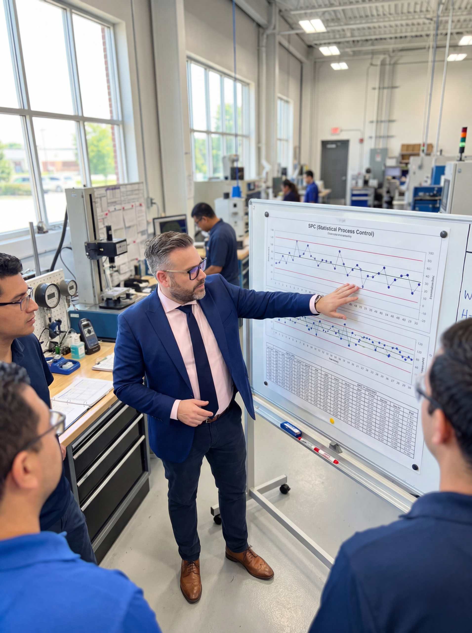
The foundational tool of SPC is the control chart, which plots process data over time against calculated statistical limits. For continuous variable data, the X̄-R (Average and Range) chart is the industry standard. The X̄ chart tracks the mean of subgroups to detect shifts in the process centre, calculated against an Upper Control Limit (UCL) and Lower Control Limit (LCL). The R chart tracks the variability within those subgroups, ensuring the process spread remains consistent.
A process is considered out of control when the data violates specific statistical rules. A single point breaching the UCL or LCL is a clear signal of instability. However, engineers must also look for underlying trends: six consecutive points steadily increasing or decreasing indicate a drift, while fourteen points alternating up and down suggest a systematic error. These rules exist because a process can be statistically unstable long before it produces a part that falls outside of engineering specifications.

During that 2008 Ford brake component project, I built an X̄-R chart to track a critical diameter. The process mean was 25.4 mm, with the UCL set at 25.6 mm. For two weeks, the data remained tightly grouped around the mean. In the third week, a measurement hit 25.55 mm, breaching the control limit. We did not wait for a defect to appear; we immediately stopped the line. Investigation revealed that the cutting tool had overheated, altering its cutting path. By enforcing a tool-cooling cycle every 200 parts, defect rates dropped from 3% to 0.2%.
Process Capability: Cp and Cpk
Control charts prove whether a process is stable over time. Process capability indices prove whether that stable process can actually meet engineering tolerances. Cp measures the potential capability, calculated by dividing the tolerance band (USL minus LSL) by the process variation (six standard deviations). However, Cp assumes the process is perfectly centred between the specification limits, which is rarely the case on a real shop floor.
Cpk addresses this limitation by factoring in the actual process mean. It calculates the distance from the process mean to the nearest specification limit, divided by three standard deviations. The automotive industry standard, dictated by IATF 16949 and PPAP requirements, demands a Cpk of 1.33 or higher for standard characteristics. For critical safety or dimensional features, the target is Cpk 1.67. A process with a Cpk of 1.0 sits exactly on the edge of the tolerance, meaning any minor shift will immediately generate non-conforming parts.
Cpk Acceptance Thresholds in Automotive and Aerospace
I once audited a drilling operation producing holes specified at 10.0 mm ± 0.2 mm. The initial Cpk was a disastrous 0.33. The process was shifted high, running at a mean of 10.12 mm. Because the mean was off-centre, the distance to the Upper Specification Limit was dangerously narrow. We corrected the tool offset, centring the process at 10.00 mm. We then addressed the variation by replacing a worn tool holder, which reduced the standard deviation from 0.08 mm to 0.04 mm. The Cpk jumped to 1.67, and the defect rate fell from 8.5% to 0.01%.
Measurement Systems Analysis (MSA) Precedes SPC
Before calculating capability indices or plotting control charts, you must prove your measurement system can reliably detect process variation. Measurement Systems Analysis (MSA), specifically Gage Repeatability and Reproducibility (GR&R), quantifies how much of the observed variation comes from the gauge and the operators rather than the parts themselves. If the gauge contributes more than 30% of the total tolerance band, any SPC data you collect is statistical noise.
A GR&R score below 10% is considered acceptable. I have seen plants proudly present capability data showing a Cpk of 2.0, only for an MSA to reveal a GR&R of 35%. The process wasn't highly capable; the operators were measuring inconsistently using a worn calibration pin and unstandardized techniques. Once the gauge was recalibrated and the measurement standard was defined, the GR&R dropped to 8%. The actual process variation was suddenly visible, and the real Cpk was barely 1.1. Trusting data from an unverified measurement system is a fundamental quality failure.
GR&R calculates the standard deviation of the measurement system and multiplies it by six, then divides that figure by the total tolerance band. Repeatability measures whether the same operator gets the same result on the same part. Reproducibility measures whether different operators get the same result on the same part. If your gauge fails these tests, your SPC charts are tracking measurement error, not process behaviour. You cannot improve a process you cannot accurately measure.
Stability Must Be Proven Before Capability
In 2015, I worked on a component line for Toyota's Hybrid Synergy Drive. The quality manager confidently informed me the process had a Cpk of 1.8. The number looked excellent on paper, but I asked to see the underlying control charts. A capability index is only valid if the process is in a state of statistical control. If you calculate Cpk on an unstable process, you are simply calculating the historical average of your chaos. The number holds no predictive value.
Stability must precede capability. A Cpk calculated on an unstable process is just the mathematical average of your chaos.
We reviewed the X̄-R charts and found a clear signal. The data had been stable for a week, but then a subgroup suddenly jumped above the UCL. The process was out of control, rendering that Cpk of 1.8 meaningless. The root cause was a change in raw material suppliers. The new batch of steel had a different hardness, which altered the stamping dynamics. The immediate fix was to revert to the qualified supplier. The systemic fix was to update the Control Plan to require supplier material verification before release to production.
The sequence matters: you must first demonstrate stability using control charts, and only then calculate capability. If a process is unstable, your engineering effort must focus on finding and eliminating the special causes of variation. Special causes are the unpredictable spikes, shifts, and trends that signal something in the process has fundamentally changed. Once those are eliminated and the process behaves consistently, you can evaluate whether your common-cause variation is tight enough to meet specifications.
Deploying SPC: Selecting the Right Charts
Effective SPC requires selecting the correct chart for the data type. Continuous variable data, such as dimensions, weights, and temperatures, requires X̄-R charts for small subgroups or X̄-s charts for larger sample sizes. If the production volume is too low to support subgrouping, an Individual-Moving Range (I-MR) chart tracks single measurements. Attribute data, which involves counting defects or defective units, requires a different approach using P, NP, C, or U charts.
The SPC Implementation Sequence
- 01Select parameterIdentify the critical characteristic that drives product quality and has clear USL/LSL tolerances.
- 02Validate measurementConduct a GR&R study. The gauge must contribute less than 10% of the tolerance to be trusted.
- 03Verify stabilityPlot the data on a control chart. Eliminate all special causes until the process is predictable.
- 04Calculate capabilityOnce stable, calculate Cp and Cpk to prove the process can meet engineering specifications.
Attribute charts track discrete events. The P chart tracks the proportion of defective units when the sample size varies, while the NP chart tracks the actual count of defective units with a constant sample size. The C chart tracks the number of defects per unit, and the U chart tracks the average defects per unit when the sample size varies. If a P chart reveals a spike in defective units at a specific hour, the root cause is often operational: a shift change, an untrained relief operator, or a machine cooldown cycle that was skipped.
Sampling frequency must match the production reality. Sampling a high-volume stamping line once per shift means you will manufacture thousands of parts between data points. If a tool breaks immediately after a sample is taken, the defect wave will not be detected until the next shift. High-volume processes require frequent subgroups—typically every 30 to 60 minutes. Low-volume processes can rely on I-MR charts. The goal is to detect a process shift before it generates significant scrap.
Common SPC Failures on the Shop Floor
The most damaging failure is recalculating specification limits to artificially inflate Cpk. When a process is incapable, some plants attempt to widen the USL and LSL rather than fix the mechanical issue. This does not improve quality; it simply redefines non-conforming parts as acceptable. The Cpk looks better on the PPAP paperwork, but the field failure rate remains unchanged. Capability indices must reflect reality, not a revised tolerance band.
Another systemic failure is ignoring out-of-control signals. When a point breaches a control limit, operators and supervisors must treat it as a mechanical alarm bell. Dismissing a breach as a one-off anomaly guarantees that the special cause will remain in the system. Every out-of-control point requires an immediate 8D root cause analysis. If the data shows a trend, the process is telling you something has changed—tool wear, thermal expansion, or material variance. You must identify and eliminate that cause before resuming production.
SPC is not limited to manufacturing geometry. The statistical principles apply to any process with variable output over time. In software development, SPC tracks API response times and error rates. In logistics, it monitors order processing times and delivery variances. In healthcare, hospitals use SPC to track patient wait times and hospital-acquired infection rates. The methodology remains identical: establish a measurement system, prove stability, and monitor for signals of unnatural variation. The goal is to replace reactive crisis management with predictable, engineered outcomes.