A customer blocking an entire shipment of critical modules focuses the mind. I have lived through this scenario: three consecutive batches rejected for systematic dimensional shift, despite every Shewhart control chart assuring us the process was stable. The standard SPC tools were technically correct, but they were answering the wrong question.
Shewhart charts are designed to catch catastrophic, sudden failures. They are blind to the slow, incremental machine drift that destroys capability over months. When a critical dimension shifts by fractions of a micron every cycle, individual measurements remain well within specification limits, but the cumulative effect pushes entire batches toward the tolerance boundary.
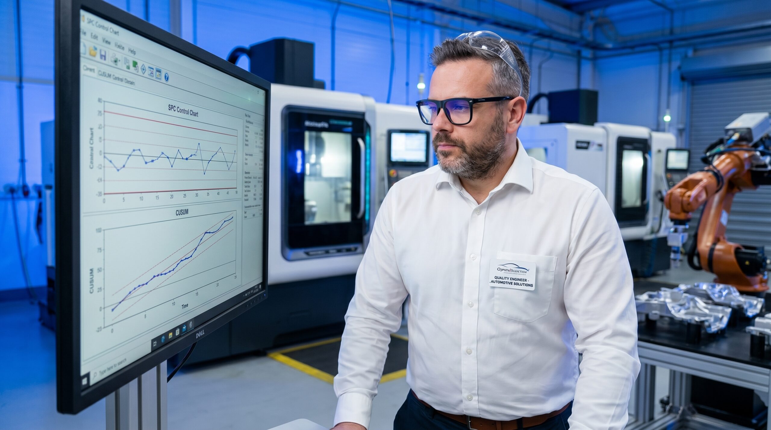
Cumulative Sum (CUSUM) methodology exposes this hidden drift. Instead of plotting individual measurements against control limits, CUSUM plots the running total of deviations from the target value. It is mathematically simpler than advanced forecasting, yet it detects small, sustained shifts two to four times faster than traditional X-bar charts.
The Mechanism: Accumulating Deviations
CUSUM does not replace your Shewhart charts; it complements them. You set a target value (T), usually the exact centre of the tolerance band. For every measurement, you calculate the deviation from that target. The algorithm then accumulates these deviations over time.
When a process runs purely on target, positive and negative deviations cancel each other out. The CUSUM curve meanders horizontally around zero. The moment the process mean shifts, even slightly, one sign begins to dominate. The curve embarks on a distinct upward or downward trajectory, signalling a sustained change in the process mean.
This trajectory is the core diagnostic signal. A standard control chart looks at each data point in isolation. CUSUM looks at the process's history, mathematically linking yesterday's production to today's output to identify trends that remain invisible to point-by-point analysis.
Implementing the Tabular CUSUM Method
To deploy this in an industrial setting, you use the tabular CUSUM method. You must define two parameters: the reference value (k) and the decision interval (h). The parameter k represents half the magnitude of the shift you want to detect, typically set at 0.5σ. The parameter h dictates the alarm threshold, usually set at 4σ or 5σ.

Tabular CUSUM Setup Sequence
- 01Define Target (T)Set to the mathematical centre of the tolerance band for symmetric specifications.
- 02Set Reference Value (k)Calculate as half the shift size you need to catch. Use 0.5σ for high sensitivity.
- 03Calculate Sums (Sᵢ)Track Upper (Sₕ) and Lower (Sₗ) cumulative sums independently using max/min logic.
- 04Trigger Alarm at hIf Sᵢ exceeds the decision interval h, stop the process and investigate.
The tabular method calculates two separate sums. The Upper CUSUM (Sₕ) tracks positive shifts using the formula: Sₕᵢ = max(0, Sₕᵢ₋₁ + (xᵢ − T) − k). The Lower CUSUM (Sₗ) tracks negative shifts: Sₗᵢ = min(0, Sₗᵢ₋₁ + (xᵢ − T) + k). When the process is stable, both values hover near zero.
When Sₕ exceeds the positive threshold +h, or Sₗ drops below the negative threshold −h, the process is officially out of control. The reaction plan in your Control Plan must dictate immediate containment and investigation, exactly as it would for a standard SPC limit breach.
Real-World Failure Mode: Undetectable Tool Wear
I investigated a case where a critical 42.00 mm module dimension systematically drifted toward the upper limit over six months. The root cause was traced to a replaced guide insert on a machining centre. The new insert, sourced to the exact same part number, had a marginally different contact surface geometry.
The deviation was approximately +0.003 mm per piece. Three microns is practically invisible on a standard Shewhart chart with a tolerance band of 0.10 mm. However, over thousands of parts, this slight geometric variance accumulated into a significant batch-level shift. The customer received product that, while technically in spec, clustered dangerously at the high limit.
A retrospective CUSUM analysis of the 14,000 data points revealed the drift began the exact week the insert was changed. Shewhart missed it entirely. The solution required reverting to the proven insert revision and adding the CUSUM algorithm to the live MES monitoring system for that specific machine.
CUSUM versus EWMA for SPC Compliance
IATF 16949 demands statistical process control for special characteristics, and the AIAG SPC manual explicitly recognises CUSUM and Exponentially Weighted Moving Average (EWMA) for detecting small shifts. Premium OEMs often mandate these advanced methods directly in their supplier Control Plans for safety-critical dimensions.
| Criterion | CUSUM | EWMA |
|---|---|---|
| Core Principle | Cumulates deviations from target | Weighted average with decaying memory |
| Best Application | Sustained step changes | Slow, continuous drift |
| Implementation | Simple max/min logic table | Requires calculating exponential weights |
| Signal Clarity | Excellent directional indication | Good, but smoothed |
For discrete manufacturing in automotive and aerospace, CUSUM is generally easier to implement and interpret. Plant engineers understand cumulative sums intuitively. EWMA is highly effective in continuous process industries like chemicals or coatings, where drift is a function of continuous flow rather than discrete cycles.
Limitations and Prerequisites for Application
CUSUM is not a universal remedy. It requires a foundational level of process stability. If your process operates with a Cpk below 0.67, you do not have a drift problem; you have a chaos problem. Implementing CUSUM on an inherently unstable process generates noise and masks the actual systemic failures.
If your process operates with a Cpk below 0.67, you do not have a drift problem; you have a chaos problem.
The mathematics assume approximate normality. For highly skewed data, such as surface flatness or coating thickness, raw CUSUM will produce false alarms. You must either transform the data to achieve normality or apply a non-parametric approach. Furthermore, CUSUM detects sustained mean shifts, not individual outliers. You still need Shewhart logic to catch a single bad part.
Finally, the algorithm needs a reliable baseline. You cannot calculate meaningful sigma values without stable historical data. If your measurement system itself is drifting due to poor gauge R&R, CUSUM will faithfully track the gauge's failure, not the machine's. Validate your MSA before trusting the algorithm.
Deploying CUSUM in the Industry 4.0 Context
Modern manufacturing removes the manual calculation burden. When 100% inspection is available, measurement data flows directly from the gauge into the Manufacturing Execution System (MES). The CUSUM algorithm runs silently in the background, evaluating the cumulative sum in real time.
Shewhart vs CUSUM Detection Capability
Shewhart Chart Behaviour
- Evaluates each point independently
- Misses incremental tool wear
- Best for sudden, gross failures
- Shows false stability during slow drift
CUSUM Chart Behaviour
- Evaluates historical process memory
- Detects sub-sigma shifts rapidly
- Best for tracking degradation
- Flags the exact week a change occurs
When the cumulative sum breaches the decision interval, the MES pushes an alert to the operator's tablet before the non-conforming part even leaves the station. This allows for immediate machine stops, tool changes, or fixture inspections. The mathematics dates to 1954, but the deployment speed is entirely modern.
Technology delivers the signal, but interpretation remains a human responsibility. The chart will tell you the process mean shifted on Tuesday at 14:00. It will not tell you why. Determining the root cause requires walking the floor, checking maintenance logs, and understanding the physics of the manufacturing process.