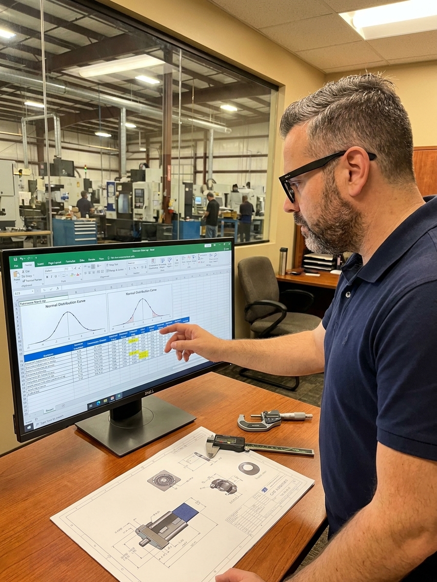
Tolerances lie in the way they interact, stack, and accumulate into variations nobody actually calculated. The drawing says each dimension is within spec. The assembly does not fit. The customer returns the lot. Nobody can explain the gap between the planned mathematics and the physical hardware.
This is the failure point that statistical tolerance analysis was built to bridge. It is also the exact point where most manufacturing organisations generate false confidence. They arm an engineer with a spreadsheet and a normal distribution assumption, then act as if the resulting calculation guarantees physical assembly success.
Over two decades of implementing IATF 16949 and AS9100 quality systems, I have audited plants where the entire scrap problem originated from an unvalidated tolerance stack-up. Teams defend against statistical ghosts, or they ignore correlated variations entirely. Fixing this requires understanding what each analytical method actually does, where its assumptions break down, and how to enforce a lifecycle management process for engineering tolerances.
The mechanics of the worst-case trap
Worst-case tolerance analysis is arithmetic addition. An engineer takes a drawing, identifies the dimensions in the stack-up chain, and sums the tolerance bands. If ten dimensions each carry a tolerance of ±0.1 mm, the worst-case total variation is ±1.0 mm. The design team either adjusts the nominal or tightens the component tolerances until the arithmetic works.
The mechanical flaw is the assumption that every dimension simultaneously hits its extreme limit, in the same direction, on the same part. In a ten-dimension stack-up, this demands a probability scenario roughly equivalent to flipping ten coins and getting heads on all ten. It can happen. It is not going to happen on any statistically capable production line.
The consequence is over-engineering. Tolerances get tightened far beyond what the process actually requires to function. Manufacturing costs rise because you are holding precision that guards against a mathematical impossibility. When someone finally questions why a non-critical dimension is held to ±0.02 mm, the justification is buried in a spreadsheet saved to a network drive three engineers ago.
Worst-case analysis has a legitimate function, but applying it blindly to every multi-component assembly drives unnecessary cost. It forces operations to expend machine time, tooling life, and operator effort hitting targets that deliver zero functional value to the end user or the next assembly stage.
Root Sum Square and the normal distribution assumption
Statistical tolerance analysis—often called Root Sum Square (RSS)—shifts the engineering question. Instead of calculating the worst possible combination of extremes, it calculates the likely distribution of assembly dimensions given the component distributions. If the variance of individual components adds up, the resulting assembly distribution predicts real-world yield.

The mathematics are straightforward. The standard deviation of the assembly is the root sum square of the individual standard deviations. This assumes a process running at a minimum capability of Cpk 1.0. From there, you calculate the probability of the assembly falling outside specification. A process running at Cpk 1.33 produces parts clustered tightly around the nominal, making the probability of all parts hitting their upper limit simultaneously vanishingly small.
RSS typically delivers a stack-up tolerance 30% to 70% smaller than the worst-case result. For a ten-dimension stack-up with equal tolerances, the RSS result is roughly one-third of the arithmetic worst-case. This translates directly into looser component tolerances, lower manufacturing costs, and higher yields. It is the difference between a profitable product and one that bleeds money on every unit.
But RSS relies on three rigid assumptions: normal distributions, independent dimensions, and centred processes. Many manufacturing engineers apply RSS across the board without verifying these conditions. They treat the statistical reduction as a mathematical shortcut rather than a conditional model. When those conditions are not met, the analysis outputs precise numbers that are systematically wrong.
Where statistical tolerance analysis fails
The first failure point is non-normal data. RSS assumes component dimensions follow a normal distribution. Machining operations often do. Sheet metal forming skews. Casting dimensions cluster at one end of the tolerance band. Additive manufacturing produces distributions that are entirely irregular. Applying RSS to skewed data yields results that look precise but are wrong in a direction you cannot predict without measuring the true distribution.
The second failure point is correlated dimensions. The RSS formula assumes statistical independence between components. In reality, a casting datum surface that is off-nominal shifts every dimension referenced from that datum in the same direction. Tool wear shifts dimensions systematically. When dimensions are positively correlated, RSS underestimates the assembly variation. Your analysis predicts 99.9% yield, but reality delivers 97%.
The third failure point is process drift. The simple RSS calculation assumes each process is centred on the nominal dimension. Tool wear pushes means. Setup variation shifts process centres between batches. Supplier changes alter the distribution entirely. A process with a Cpk of 1.33 but a Cpu of 0.8 because the mean has shifted is not the benign scenario your spreadsheet assumes.
A Monte Carlo simulation fed with guesses is not analysis. It is theatre with decimals.
Monte Carlo simulation and the data requirement
Monte Carlo tolerance analysis replaces the analytical RSS calculation with brute-force computational simulation. Instead of assuming normal distributions and independence, you define each dimension with its actual measured distribution, including correlations, shifts, and drifts. You simulate the assembly thousands of times, drawing random values to generate a true distribution curve.
The advantage of Monte Carlo is absolute flexibility. It handles non-normal distributions, correlated dimensions, shifted processes, non-linear stack-ups, and complex geometric tolerancing scenarios under AS9100 or IATF 16949 requirements. The disadvantage is that it demands real statistical process control data—not just tolerance bands from a drawing.
Selecting the correct tolerance analysis method
- 01Worst-Case AnalysisApply when failure is catastrophic, volume is low (<1,000 units), or the stack-up is three dimensions or fewer.
- 02RSS MethodApply when there are four or more dimensions from capable, independent, approximately normal processes (Cpk ≥ 1.33).
- 03Monte Carlo SimulationApply for complex GD&T, known non-normal distributions, correlated datums, and high-volume production (>10,000 units).
Most organisations are not ready for Monte Carlo because their data infrastructure is missing. Running a meaningful simulation requires knowing the actual mean, standard deviation, skewness, and kurtosis of each manufacturing step. Without that high-resolution SPC data, the simulation degrades into guessing distributions instead of measuring them.
The organisational failure mode
The pattern repeats across automotive and aerospace plants. A design engineer performs a tolerance analysis early in development using nominal dimensions and standard defaults. The analysis shows the design works. The engineer files the document and moves to the next task. The analysis is treated as a checkbox, not a living engineering document.
Six months later, manufacturing reports that 3% of assemblies fail specification. Quality traces the problem to tolerance accumulation across three supplier-provided components. The retrieved tolerance analysis reveals it assumed ±0.05 mm on those dimensions. The drawing was released at ±0.1 mm because the supplier could not meet the tighter spec. Nobody updated the analysis.
This is not a failure of statistical mathematics. It is a failure of process discipline. When tolerances changed, nobody re-ran the analysis. When the supplier changed, nobody updated the distribution assumptions. When the process drifted on the floor, nobody measured the impact on the final assembly yield.
Building a functional tolerance management process means assigning single-point ownership for each stack-up. The analysis must live inside the product data management system, tied directly to CAD models. When a drawing changes, the change order mandates a tolerance review. Tolerance management becomes a lifecycle activity, not a milestone deliverable for a design review gate.
Closing the loop with validation studies
No analytical method works without physical validation. Whatever your tolerance analysis predicts—worst-case, RSS, or Monte Carlo—the only way to verify it is to measure actual assemblies and compare the data to the predictions. This is a tolerance validation study, and it is the step most organisations systematically skip.
Key thresholds for capable tolerance management
Before a product moves from pilot to full production, measure a statistically significant sample of assemblies. If the predicted yield does not match the physical measurements, correct the analysis before scaling. This validation must be a mandatory gate in the APQP or PPAP process, not an optional engineering exercise.
The quality organisation must maintain a live database of process capability for each manufacturing operation and supplier. This database replaces the default tolerance-divided-by-three assumption with real standard deviations. When field failures or in-process defects trace back to tolerance issues, the 8D investigation must force an update to the original tolerance model.
Organisations that manage tolerances well are not using better math; they are applying better discipline. The difference between a plant that spends 15% of product cost on scrap and one that spends 3% is not analytical sophistication. It is the operational rigour to ask whether a process can hold a tolerance before the drawing is released, not after the first lot fails.