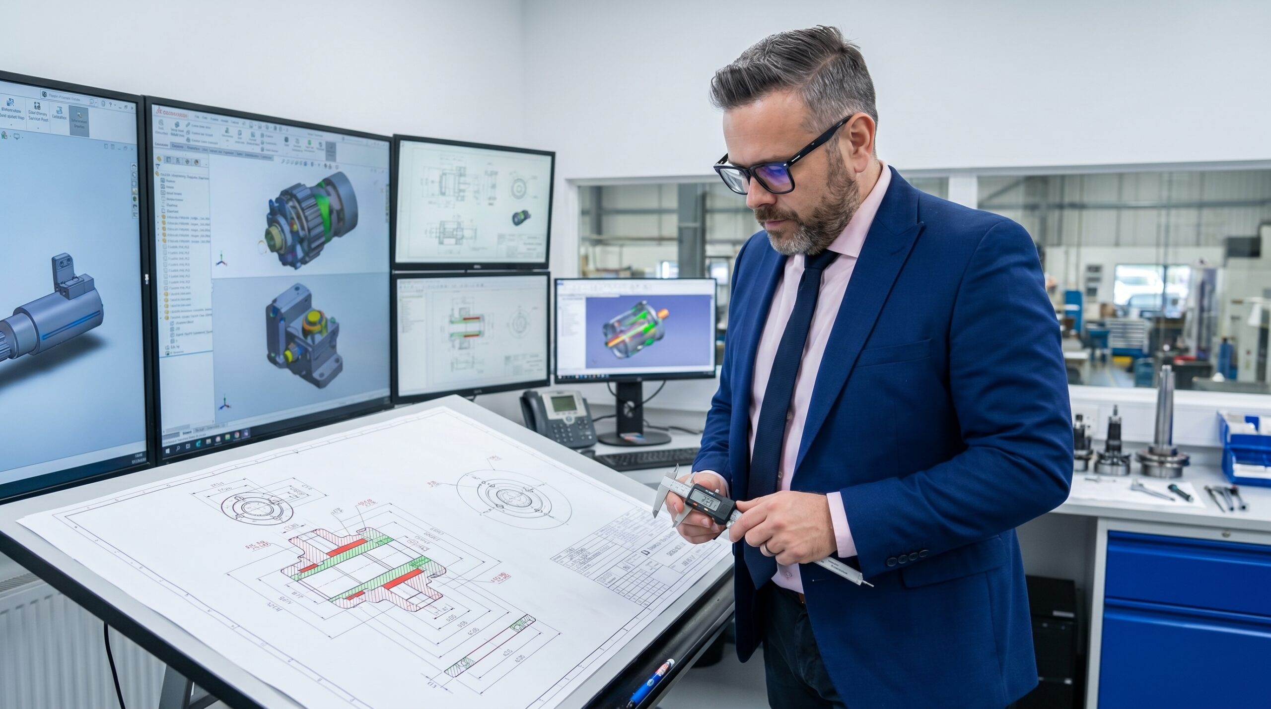
A process engineer once walked into my office holding three machined parts. All three were within their drawing tolerances. Together, they would not fit into the assembly. Management was registering the rejection as supplier defect; we were calling it a fundamental misunderstanding of stack-up.
Every individual dimension was correct in isolation. Nobody had calculated what happens when all three tolerances converge at a single assembly point. That day, tolerance analysis became a mandatory step for every new product introduction in our facility.
Tolerance analysis replaces guesswork with calculation. It dictates whether you run a cost-effective process or fight a losing battle against scrap, rework, and machines incapable of holding the specified limits.
How Engineers Assign Tolerances
Most design engineers assign tolerances using one of three flawed approaches. They copy defaults from previous projects, set limits based purely on machine capability, or apply overly tight values out of caution.
Copying from past drawings propagates historical errors. Tightening tolerances to ±0.005 mm for safety increases manufacturing costs exponentially and often demands specialised operations that disrupt flow. Tolerance analysis forces the engineering team to justify every decimal place.
Tolerance Assignment: Guesswork vs Calculation
What teams do
- Copy ±0.1 mm from a legacy drawing without review.
- Tighten to ±0.005 mm 'just to be safe' during design.
- Ignore cumulative stack-up effects across the assembly.
- Wait for the prototype build to discover interference.
What works
- Calculate the RSS or worst-case limit for the chain.
- Set limits based on functional requirements and process data.
- Widen non-critical dimensions to optimise machining costs.
- Validate the model using 30-50 physical measurements.
Worst-Case vs Statistical Analysis
When you face a dimension chain, you have two primary calculation methods. Worst-Case Analysis assumes all parts land simultaneously at the extreme limits of their tolerances. Mathematically, the assembly tolerance equals the arithmetic sum of individual tolerances.
If you have three parts with a tolerance of ±0.1 mm, the worst-case assembly tolerance is ±0.3 mm. This method offers an absolute guarantee: if parts meet specification, the assembly fits. The penalty is over-engineering.
Statistical tolerance analysis — specifically the Root Sum of Squares (RSS) method — reflects manufacturing reality. It assumes dimensions are normally distributed and independent. The formula calculates the square root of the sum of squared individual tolerances.
Applying RSS to those same three parts (±0.1 mm) yields an assembly tolerance of approximately ±0.173 mm. This statistical approach proves you can safely widen individual component tolerances while maintaining assembly function, drastically reducing cost.
Method Selection Matrix
| Situation | Recommended Method | Rationale |
|---|---|---|
| Critical safety (aerospace, medical) | Worst-Case | No statistical risk accepted |
| 3 or fewer dimensions in chain | Worst-Case | Statistical benefit is negligible |
| 4+ independent dimensions | RSS | Statistics favourably reduce the stack-up |
| Dependent variables (shared fixture) | Monte Carlo | RSS gives false confidence with correlations |
| High-volume, capable process | RSS with Cpk validation | Best ratio of cost to reliability |
Monte Carlo simulation is the third option. Instead of analytical formulas, the software generates thousands of virtual assemblies, drawing randomly from the actual distribution of each dimension. This approach is essential for complex mechanisms with non-linear relationships or correlated variables machined in a single setup.

Validating the Chain in Production
I ran a tolerance analysis on an electrical contactor for a battery module. The assembly contained seven dimensions defining the critical air gap between contacts. The safety window was tight: 1.8 mm to 2.2 mm.
The original design specified ±0.02 mm for every dimension. Production was choking. Operators measured every piece under a microscope, tooling wore out rapidly, and the scrap rate was climbing. We stopped production and analysed the chain.
Tolerance Analysis Workflow
- 01Map the chainDraw the 1D or 3D loop from the datum to the functional gap.
- 02Gather real dataMeasure 30-50 actual parts to calculate mean, sigma, and Cpk.
- 03Calculate the stack-upRun RSS or Monte Carlo using the measured distributions.
- 04Optimise limitsWiden non-critical tolerances and tighten the true constraints.
We pulled 50 parts from the line and measured them. Three dimensions had a Cpk exceeding 2.0, meaning the process was vastly better than the drawing required. Two dimensions sat at a Cpk of 1.33. Two dimensions were borderline at a Cpk of 1.0.
We ran the RSS calculation using the real standard deviations. The model showed that 99.97% of assemblies would meet the air gap requirement. The problem was not the tolerances themselves, but a mean shift on one dimension that was running off-centre.
We widened three non-critical tolerances from ±0.02 mm to ±0.05 mm. We tightened the one dimension driving the failure and centred the process. Machining costs dropped by 23%, scrap fell from 2.1% to 0.3%, and the line speed increased by 15% due to fewer tool changes.
Common Failure Modes
The most dangerous trap is ignoring dependencies between dimensions. If two features are machined in a single setup, they are not independent. Applying RSS to correlated variables produces a falsely optimistic result. Use Monte Carlo with a correlation matrix, or model the difference between the dimensions directly.
Teams frequently model only a 1D chain when the physical assembly is 3D. Angularity, perpendicularity, and lateral influences destroy 1D assumptions. Complex assemblies require 3D tolerance analysis software like 3DCS, VisVSA, or CETOL.
Working with drawing tolerances instead of real production data is another error. The drawing is a contract, not a forecast. Actual distributions can be wider, narrower, shifted, or bimodal. Always feed actual SPC data into the analysis.
A drawing tolerance is a contract; the production distribution is the reality that actually dictates your scrap rate.
Finally, neglecting thermal and mechanical effects invalidates static models. Dimensions measured at 20°C behave differently at 80°C operating temperature. Include coefficients of thermal expansion in the stack-up.
Integration with APQP and PPAP
In IATF 16949 environments, tolerance analysis is mandatory within Advanced Product Quality Planning (APQP). It functions as the primary input for Design FMEAs during Phase 2 and dictates what the manufacturing process must capable of holding in Phase 3.
During PPAP submission, the tolerance study must be validated against actual production runs. I have reviewed PPAP packages where the tolerance analysis was a pristine Excel file that had never seen a single measurement from the floor. If you are the supplier, execute the validation study. If you are the auditor, demand the measurement data.
Six Sigma and Variance Contribution
Tolerance analysis integrates tightly with Six Sigma DMAIC. By calculating the percentage contribution of each dimension to the total assembly variance, you know exactly where to direct improvement resources.
If Dimension A contributes 60% of the variance and Dimension B contributes 5%, tightening Dimension B is wasted effort. This sensitivity analysis applies Taguchi's philosophy: hold tight tolerances only where variation causes functional pain.
Tools and Software
You can execute a basic RSS calculation in Excel using the formula =SQRT(SUMSQ(range)). For advanced statistical integration, Minitab and JMP offer dedicated modules.
For complex 3D mechanisms, CETOL 6σ integrates directly with CAD software. 3DCS by Dassault Systèmes handles large automotive assemblies, and Enventive combines mechanical design computation with tolerance optimisation.
Software is a calculator. The engineering decision regarding which method to apply, whether the statistical assumptions hold, and what the results mean for the production line remains the responsibility of the quality and engineering teams.
Regarding the three parts that started this discussion: the drawing tolerance was symmetrical at ±0.05 mm, but the manufacturing process was shifted by +0.03 mm. The parts were compliant on paper but systematically at the boundary in reality. We re-centred the process, the assembly closed, and the Friday afternoon crisis ended.